

My reaction when I first came across the terms counter and gauge and the graphs with colors and numbers labeled "mean" and "upper 90" was one of avoidance. It's like I saw them, but I didn't care because I didn't understand them or how they might be useful. Since my job didn't require me to pay attention to them, they remained ignored.
That was about two years ago. As I progressed in my career, I wanted to understand more about our network applications, and that is when I started learning about metrics.
The three stages of my journey to understanding monitoring (so far) are:
- Stage 1: What? (Looks elsewhere)
- Stage 2: Without metrics, we are really flying blind.
- Stage 3: How do we keep from doing metrics wrong?
I am currently in Stage 2 and will share what I have learned so far. I'm moving gradually toward Stage 3, and I will offer some of my resources on that part of the journey at the end of this article.
Let's get started!
Software prerequisites
All the demos discussed in this article are available on my GitHub repo. You will need to have docker and docker-compose installed to play with them.
Why should I monitor?
The top reasons for monitoring are:
- Understanding normal and abnormal system and service behavior
- Doing capacity planning, scaling up or down
- Assisting in performance troubleshooting
- Understanding the effect of software/hardware changes
- Changing system behavior in response to a measurement
- Alerting when a system exhibits unexpected behavior
Metrics and metric types
For our purposes, a metric is an observed value of a certain quantity at a given point in time. The total of number hits on a blog post, the total number of people attending a talk, the number of times the data was not found in the caching system, the number of logged-in users on your website—all are examples of metrics.
They broadly fall into three categories:
Counters
Consider your personal blog. You just published a post and want to keep an eye on how many hits it gets over time, a number that can only increase. This is an example of a counter metric. Its value starts at 0 and increases during the lifetime of your blog post. Graphically, a counter looks like this:
opensource.com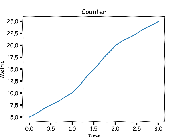
Gauges
Instead of the total number of hits on your blog post over time, let's say you want to track the number of hits per day or per week. This metric is called a gauge and its value can go up or down. Graphically, a gauge looks like this:
opensource.com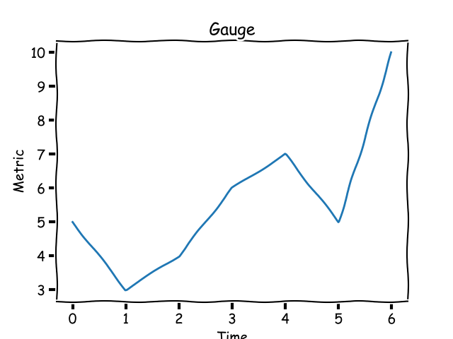
A gauge's value usually has a ceiling and a floor in a certain time window.
Histograms and timers
A histogram (as Prometheus calls it) or a timer (as StatsD calls it) is a metric to track sampled observations. Unlike a counter or a gauge, the value of a histogram metric doesn't necessarily show an up or down pattern. I know that doesn't make a lot of sense and may not seem different from a gauge. What's different is what you expect to do with histogram data compared to a gauge. Therefore, the monitoring system needs to know that a metric is a histogram type to allow you to do those things.
opensource.com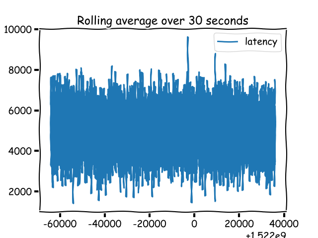
Demo 1: Calculating and reporting metrics
Demo 1 is a basic web application written using the Flask framework. It demonstrates how we can calculate and report metrics.
The src directory has the application in app.py with the src/helpers/middleware.py containing the following:
from flask import request
import csv
import time


def start_timer():
    request.start_time = time.time()


def stop_timer(response):
    # convert this into milliseconds for statsd
    resp_time = (time.time() - request.start_time)*1000
    with open('metrics.csv', 'a', newline='') as f:
        csvwriter = csv.writer(f)
        csvwriter.writerow([str(int(time.time())), str(resp_time)])

    return response


def setup_metrics(app):
    app.before_request(start_timer)
    app.after_request(stop_timer)
When setup_metrics() is called from the application, it configures the start_timer() function to be called before a request is processed and the stop_timer() function to be called after a request is processed but before the response has been sent. In the above function, we write the timestamp and the time it took (in milliseconds) for the request to be processed.
When we run docker-compose up in the demo1 directory, it starts the web application, then a client container that makes a number of requests to the web application. You will see a src/metrics.csv file that has been created with two columns: timestamp and request_latency.
Looking at this file, we can infer two things:
- There is a lot of data that has been generated
- No observation of the metric has any characteristic associated with it
Without a characteristic associated with a metric observation, we cannot say which HTTP endpoint this metric was associated with or which node of the application this metric was generated from. Hence, we need to qualify each metric observation with the appropriate metadata.
Statistics 101
If we think back to high school mathematics, there are a few statistics terms we should all recall, even if vaguely, including mean, median, percentile, and histogram. Let's briefly recap them without judging their usefulness, just like in high school.
Mean
The mean, or the average of a list of numbers, is the sum of the numbers divided by the cardinality of the list. The mean of 3, 2, and 10 is (3+2+10)/3 = 5.
Median
The median is another type of average, but it is calculated differently; it is the center numeral in a list of numbers ordered from smallest to largest (or vice versa). In our list above (2, 3, 10), the median is 3. The calculation is not very straightforward; it depends on the number of items in the list.
Percentile
The percentile is a measure that gives us a measure below which a certain (k) percentage of the numbers lie. In some sense, it gives us an idea of how this measure is doing relative to the k percentage of our data. For example, the 95th percentile score of the above list is 9.29999. The percentile measure varies from 0 to 100 (non-inclusive). The zeroth percentile is the minimum score in a set of numbers. Some of you may recall that the median is the 50th percentile, which turns out to be 3.
Some monitoring systems refer to the percentile measure as upper_X where X is the percentile; upper 90 refers to the value at the 90th percentile.
Quantile
The q-Quantile is a measure that ranks qN in a set of N numbers. The value of q ranges between 0 and 1 (both inclusive). When q is 0.5, the value is the median. The relationship between the quantile and percentile is that the measure at q quantile is equivalent to the measure at 100q percentile.
Histogram
The metric histogram, which we learned about earlier, is an implementation detail of monitoring systems. In statistics, a histogram is a graph that groups data into buckets. Let's consider a different, contrived example: the ages of people reading your blog. If you got a handful of this data and wanted a rough idea of your readers' ages by group, plotting a histogram would show you a graph like this:
opensource.com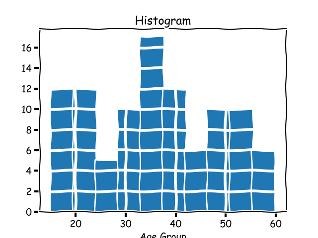
Cumulative histogram
A cumulative histogram is a histogram where each bucket's count includes the count of the previous bucket, hence the name cumulative. A cumulative histogram for the above dataset would look like this:
opensource.com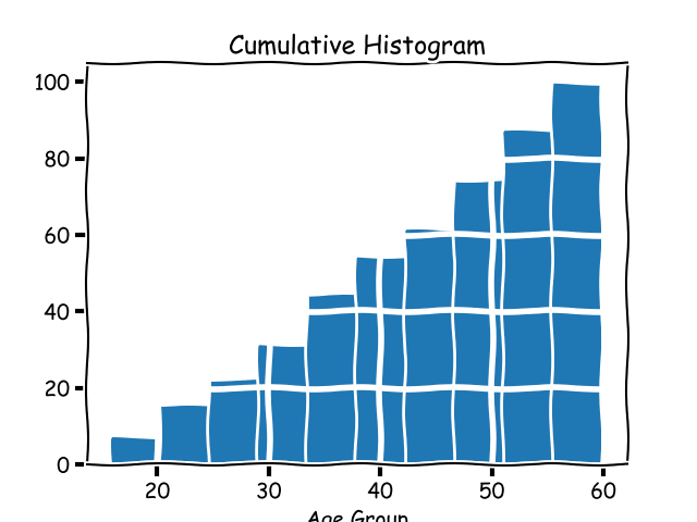
Why do we need statistics?
In Demo 1 above, we observed that there is a lot of data that is generated when we report metrics. We need statistics when working with metrics because there are just too many of them. We don't care about individual values, rather overall behavior. We expect the behavior the values exhibit is a proxy of the behavior of the system under observation.
Demo 2: Adding characteristics to metrics
In our Demo 1 application above, when we calculate and report a request latency, it refers to a specific request uniquely identified by few characteristics. Some of these are:
- The HTTP endpoint
- The HTTP method
- The identifier of the host/node where it's running
If we attach these characteristics to a metric observation, we have more context around each metric. Let's explore adding characteristics to our metrics in Demo 2.
The src/helpers/middleware.py file now writes multiple columns to the CSV file when writing metrics:
node_ids = ['10.0.1.1', '10.1.3.4']


def start_timer():
    request.start_time = time.time()


def stop_timer(response):
    # convert this into milliseconds for statsd
    resp_time = (time.time() - request.start_time)*1000
    node_id = node_ids[random.choice(range(len(node_ids)))]
    with open('metrics.csv', 'a', newline='') as f:
        csvwriter = csv.writer(f)
        csvwriter.writerow([
            str(int(time.time())), 'webapp1', node_id,
            request.endpoint, request.method, str(response.status_code),
            str(resp_time)
        ])

    return response
Since this is a demo, I have taken the liberty of reporting random IPs as the node IDs when reporting the metric. When we run docker-compose up in the demo2 directory, it will result in a CSV file with multiple columns.
Analyzing metrics with pandas
We'll now analyze this CSV file with pandas. Running docker-compose up will print a URL that we will use to open a Jupyter session. Once we upload the Analysis.ipynb notebook into the session, we can read the CSV file into a pandas DataFrame:
import pandas as pd
metrics = pd.read_csv('/data/metrics.csv', index_col=0)
The index_col specifies that we want to use the timestamp as the index.
Since each characteristic we add is a column in the DataFrame, we can perform grouping and aggregation based on these columns:
import numpy as np
metrics.groupby(['node_id', 'http_status']).latency.aggregate(np.percentile, 99.999)
Please refer to the Jupyter notebook for more example analysis on the data.
What should I monitor?
A software system has a number of variables whose values change during its lifetime. The software is running in some sort of an operating system, and operating system variables change as well. In my opinion, the more data you have, the better it is when something goes wrong.
Key operating system metrics I recommend monitoring are:
- CPU usage
- System memory usage
- File descriptor usage
- Disk usage
Other key metrics to monitor will vary depending on your software application.
Network applications
If your software is a network application that listens to and serves client requests, the key metrics to measure are:
- Number of requests coming in (counter)
- Unhandled errors (counter)
- Request latency (histogram/timer)
- Queued time, if there is a queue in your application (histogram/timer)
- Queue size, if there is a queue in your application (gauge)
- Worker processes/threads usage (gauge)
If your network application makes requests to other services in the context of fulfilling a client request, it should have metrics to record the behavior of communications with those services. Key metrics to monitor include number of requests, request latency, and response status.
HTTP web application backends
HTTP applications should monitor all the above. In addition, they should keep granular data about the count of non-200 HTTP statuses grouped by all the other HTTP status codes. If your web application has user signup and login functionality, it should have metrics for those as well.
Long-running processes
Long-running processes such as Rabbit MQ consumer or task-queue workers, although not network servers, work on the model of picking up a task and processing it. Hence, we should monitor the number of requests processed and the request latency for those processes.
No matter the application type, each metric should have appropriate metadata associated with it.
Integrating monitoring in a Python application
There are two components involved in integrating monitoring into Python applications:
- Updating your application to calculate and report metrics
- Setting up a monitoring infrastructure to house the application's metrics and allow queries to be made against them
The basic idea of recording and reporting a metric is:
def work():
    requests += 1
    # report counter
    start_time = time.time()

    # < do the work >

    # calculate and report latency
    work_latency = time.time() - start_time
    ...
Considering the above pattern, we often take advantage of decorators, context managers, and middleware (for network applications) to calculate and report metrics. In Demo 1 and Demo 2, we used decorators in a Flask application.
Pull and push models for metric reporting
Essentially, there are two patterns for reporting metrics from a Python application. In the pull model, the monitoring system "scrapes" the application at a predefined HTTP endpoint. In the push model, the application sends the data to the monitoring system.
opensource.com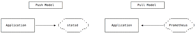
An example of a monitoring system working in the pull model is Prometheus. StatsD is an example of a monitoring system where the application pushes the metrics to the system.
Integrating StatsD
To integrate StatsD into a Python application, we would use the StatsD Python client, then update our metric-reporting code to push data into StatsD using the appropriate library calls.
First, we need to create a client instance:
statsd = statsd.StatsClient(host='statsd', port=8125, prefix='webapp1')The prefix keyword argument will add the specified prefix to all the metrics reported via this client.
Once we have the client, we can report a value for a timer using:
statsd.timing(key, resp_time)To increment a counter:
statsd.incr(key)
To associate metadata with a metric, a key is defined as metadata1.metadata2.metric, where each metadataX is a field that allows aggregation and grouping.
The demo application StatsD is a complete example of integrating a Python Flask application with statsd.
Integrating Prometheus
To use the Prometheus monitoring system, we will use the Promethius Python client. We will first create objects of the appropriate metric class:
REQUEST_LATENCY = Histogram('request_latency_seconds', 'Request latency',
    ['app_name', 'endpoint']
)
The third argument in the above statement is the labels associated with the metric. These labels are what defines the metadata associated with a single metric value.
To record a specific metric observation:
REQUEST_LATENCY.labels('webapp', request.path).observe(resp_time)
The next step is to define an HTTP endpoint in our application that Prometheus can scrape. This is usually an endpoint called /metrics:
@app.route('/metrics')
def metrics():
    return Response(prometheus_client.generate_latest(), mimetype=CONTENT_TYPE_LATEST)
The demo application Prometheus is a complete example of integrating a Python Flask application with prometheus.
Which is better: StatsD or Prometheus?
The natural next question is: Should I use StatsD or Prometheus? I have written a few articles on this topic, and you may find them useful:
- Your options for monitoring multi-process Python applications with Prometheus
- Monitoring your synchronous Python web applications using Prometheus
- Monitoring your asynchronous Python web applications using Prometheus
Ways to use metrics
We've learned a bit about why we want to set up monitoring in our applications, but now let's look deeper into two of them: alerting and autoscaling.
Using metrics for alerting
A key use of metrics is creating alerts. For example, you may want to send an email or pager notification to relevant people if the number of HTTP 500s over the past five minutes increases. What we use for setting up alerts depends on our monitoring setup. For Prometheus we can use Alertmanager and for StatsD, we use Nagios.
Using metrics for autoscaling
Not only can metrics allow us to understand if our current infrastructure is over- or under-provisioned, they can also help implement autoscaling policies in a cloud infrastructure. For example, if worker process usage on our servers routinely hits 90% over the past five minutes, we may need to horizontally scale. How we would implement scaling depends on the cloud infrastructure. AWS Auto Scaling, by default, allows scaling policies based on system CPU usage, network traffic, and other factors. However, to use application metrics for scaling up or down, we must publish custom CloudWatch metrics.
Application monitoring in a multi-service architecture
When we go beyond a single application architecture, such that a client request can trigger calls to multiple services before a response is sent back, we need more from our metrics. We need a unified view of latency metrics so we can see how much time each service took to respond to the request. This is enabled with distributed tracing.
You can see an example of distributed tracing in Python in my blog post Introducing distributed tracing in your Python application via Zipkin.
Points to remember
In summary, make sure to keep the following things in mind:
- Understand what a metric type means in your monitoring system
- Know in what unit of measurement the monitoring system wants your data
- Monitor the most critical components of your application
- Monitor the behavior of your application in its most critical stages
The above assumes you don't have to manage your monitoring systems. If that's part of your job, you have a lot more to think about!
Other resources
Following are some of the resources I found very useful along my monitoring education journey:
General
StatsD/Graphite
Prometheus
- Prometheus metric types
- How does a Prometheus gauge work?
- Why are Prometheus histograms cumulative?
- Monitoring batch jobs in Python
- Prometheus: Monitoring at SoundCloud
Avoiding mistakes (i.e., Stage 3 learnings)
As we learn the basics of monitoring, it's important to keep an eye on the mistakes we don't want to make. Here are some insightful resources I have come across:
- How not to measure latency
- Histograms with Prometheus: A tale of woe
- Why averages suck and percentiles are great
- Everything you know about latency is wrong
- Who moved my 99th percentile latency?
- Logs and metrics and graphs
- HdrHistogram: A better latency capture method
To learn more, attend Amit Saha's talk, Counter, gauge, upper 90—Oh my!, at PyCon Cleveland 2018.


2 Comments