

In the age of high-speed internet, most large information systems are structured as distributed systems with components running on different machines. The performance of these systems is generally assessed by their throughput and response time. When performance is poor, debugging these systems is challenging due to the complex interactions between different subcomponents and the possibility of the problem occurring at various places along the communication path.
On the fastest networks, the performance of a distributed system is limited by the host's ability to generate, transmit, process, and receive data, which is in turn dependent on its hardware and configuration. What if it were possible to tune the network performance of a distributed system using a repository of network benchmark runs and suggest a subset of hardware and OS parameters that are the most effective in improving network performance?
To answer this question, our team used Pbench, a benchmarking and performance analysis framework developed by the performance engineering team at Red Hat. This article will walk step by step through our process of determining the most effective methods and implementing them in a predictive performance tuning tool.
What is the proposed approach?
Given a dataset of network benchmark runs, we propose the following steps to solve this problem.
- Data preparation: Gather the configuration information, workload, and performance results for the network benchmark; clean the data; and store it in a format that is easy to work with
- Finding significant features: Choose an initial set of OS and hardware parameters and use various feature selection methods to identify the significant parameters
- Develop a predictive model: Develop a machine learning model that can predict network performance for a given client and server system and workload
- Recommend configurations: Given the user's desired network performance, suggest a configuration for the client and the server with the closest performance in the database, along with data showing the potential window of variation in results
- Evaluation: Determine the model's effectiveness using cross-validation, and suggest ways to quantify the improvement due to configuration recommendations
We collected the data for this project using Pbench. Pbench takes as input a benchmark type with its workload, performance tools to run, and hosts on which to execute the benchmark, as shown in the figure below. It outputs the benchmark results, tool results, and the system configuration information for all the hosts.
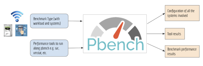
(Hifza Khalid, CC BY-SA 4.0)
Out of the different benchmark scripts that Pbench runs, we used data collected using the uperf benchmark. Uperf is a network performance tool that takes the description of the workload as input and generates the load accordingly to measure system performance.
Data preparation
There are two disjoint sets of data generated by Pbench. The configuration data from the systems under test is stored in a file system. The performance results, along with the workload metadata, are indexed into an Elasticsearch instance. The mapping between the configuration data and the performance results is also stored in Elasticsearch. To interact with the data in Elasticsearch, we used Kibana. Using both of these datasets, we combined the workload metadata, configuration data, and performance results for each benchmark run.
Finding significant features
To select an initial set of hardware specifications and operating system configurations, we used performance-tuning configuration guides and feedback from experts at Red Hat. The goal of this step was to start working with a small set of parameters and refine it with further analysis. The set was based on parameters from almost all major system subcomponents, including hardware, memory, disk, network, kernel, and CPU.
Once we selected the preliminary set of features, we used one of the most common dimensionality-reduction techniques to eliminate the redundant parameters: remove parameters with constant values. While this step eliminated some of the parameters, given the complexity of the relationship between system information and performance, we resolved to use advanced feature selection methods.
Correlation-based feature selection
Correlation is a common measure used to find the association between two features. The features have a high correlation if they are linearly dependent. If the two features increase simultaneously, their correlation is +1; if they decrease concurrently, it is -1. If the two features are uncorrelated, their correlation is close to 0.
We used the correlation between the system configuration and the target variable to identify and cut down insignificant features further. To do so, we calculated the correlation between the configuration parameters and the target variable and eliminated all parameters with a value less than |0.1|, which is a commonly used threshold to identify the uncorrelated pairs.
Feature-selection methods
Since correlation does not imply causation, we needed additional feature-selection methods to extract the parameters affecting the target variables. We could choose between wrapper methods like recursive feature elimination and embedded methods like Lasso (Least Absolute Shrinkage and Selection Operator) and tree-based methods.
We chose to work with tree-based embedded methods for their simplicity, flexibility, and low computational cost compared to wrapper methods. These methods have built-in feature selection methods. Among tree-based methods, we had three options: a classification and regression tree (CART), Random Forest, and XGBoost.
We calculated our final set of significant features for the client and server systems by taking a union of the results received from the three tree-based methods, as shown in the following table.
| Parameters | client/server | Description |
|---|---|---|
| Advertised_auto-negotation | client | If the linked advertised auto-negotiation |
| CPU(s) | server | Number of logical cores on the machine |
| Network speed | server | Speed of the ethernet device |
| Model name | client | Processor model |
| rx_dropped | server | Packets dropped after entering the computer stack |
| Model name | server | Processor model |
| System type | server | Virtual or physical system |
Develop predictive model
For this step, we used the Random Forest (RF) prediction model since it is known to perform better than CART and is also easier to visualize.
Random Forest (RF) builds multiple decision trees and merges them to get a more stable and accurate prediction. It builds the trees the same way CART does, but to ensure that the trees are uncorrelated to protect each other from their individual errors, it uses a technique known as bagging. Bagging uses random samples from the data with replacement to train the individual trees. Another difference between trees in a Random Forest and a CART decision tree is the choice of features considered for each split. CART considers every possible feature for each split. However, each tree in a Random Forest picks only from a random subset of features. This leads to even more variation among the Random Forest trees.
The RF model was constructed separately for both the target variables.
Recommend configurations
For this step, given desired throughput and response time values, along with the workload of interest, our tool searches through the database of benchmark runs to return the configuration with the performance results closest to what the user requires. It also returns the standard deviation for various samples of that run, suggesting potential variation in the actual results.
Evaluation
To evaluate our predictive model, we used a repeated K-Fold cross-validation technique. It is a popular choice to get an accurate estimate of the efficiency of the predictive model.
To evaluate the predictive model with a dataset of 9,048 points, we used k equal to 10 and repeated the cross-validation method three times. The accuracy was calculated using the two metrics given below.
- R2 score: The proportion of the variance in the dependent variable that is predictable from the independent variable(s). Its value varies between -1 and 1.
- Root mean squared error (RMSE): It measures the average squared difference between the estimated values and the actual values and returns its square root.
Based on the above two criteria, the results for the predictive model with throughput and latency as target variables are as follows:
- Throughput (trans/sec):
- R2 score: 0.984
- RMSE: 0.012
- Latency (usec):
- R2 score: 0.930
- RMSE: 0.025
What does the final tool look like?
We implemented our approach in a tool shown in the following figure. The tool is implemented in Python. It takes as input the dataset containing the information about benchmark runs as a CSV file, including client and server configuration, workload, and the desired values for latency and throughput. The tool uses this information to predict the latency and throughput results for the user's client server system. It then searches through the database of benchmark runs to return the configuration that has performance results closest to what the user requires, along with the standard deviation for that run. The standard deviation is part of the dataset and is calculated using repeated samples for one iteration or run.
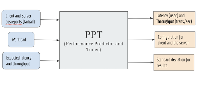
(Hifza Khalid, CC BY-SA 4.0)
What were the challenges with this approach?
While working on this problem, there were several challenges that we addressed. The first major challenge was gathering benchmark data, which required learning Elasticsearch and Kibana, the two industrial tools used by Red Hat to index, store, and interact with Pbench data. Another difficulty was dealing with the inconsistencies in data, missing data, and errors in the indexed data. For example, workload data for the benchmark runs was indexed in Elasticsearch, but one of the crucial workload parameters, runtime, was missing. For that, we had to write extra code to access it from the raw benchmark data stored on Red Hat servers.
Once we overcame the above challenges, we spent a large chunk of our effort trying out almost all the feature selection techniques available and figuring out a representative set of hardware and OS parameters for network performance. It was challenging to understand the inner workings of these techniques, their limitations, and their applications and analyze why most of them did not apply to our case. Because of space limitations and shortage of time, we did not discuss all of these methods in this article.


Comments are closed.