In the first part of this series, we looked at advances in leveraging the power of relational databases "at scale" using Apache Spark SQL and DataFrames. We will now do a simple tutorial based on a real-world dataset to look at how to use Spark SQL. We will be using Spark DataFrames, but the focus will be more on using SQL. In a separate article, I will cover a detailed discussion around Spark DataFrames and common operations.
I love using cloud services for my machine learning, deep learning, and even big data analytics needs, instead of painfully setting up my own Spark cluster. I will be using the Databricks Platform for my Spark needs. Databricks is a company founded by the creators of Apache Spark that aims to help clients with cloud-based big data processing using Spark.
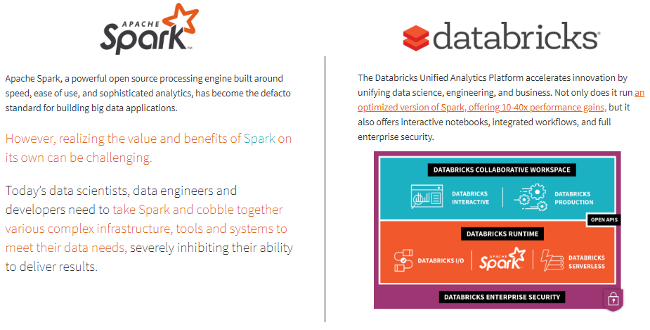
The simplest (and free of charge) way is to go to the Try Databricks page and sign up for a community edition account. You get a cloud-based cluster, which is a single-node cluster with 6GB and unlimited notebooks—not bad for a free version! I recommend using the Databricks Platform if you have serious needs for analyzing big data.
Let's get started with our case study now. Feel free to create a new notebook from your home screen in Databricks or your own Spark cluster.
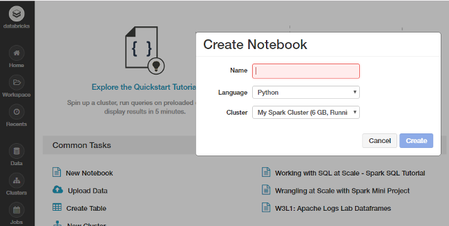
You can also import my notebook containing the entire tutorial, but please make sure to run every cell and play around and explore with it, instead of just reading through it. Unsure of how to use Spark on Databricks? Follow this short but useful tutorial.
This tutorial will familiarize you with essential Spark capabilities to deal with structured data often obtained from databases or flat files. We will explore typical ways of querying and aggregating relational data by leveraging concepts of DataFrames and SQL using Spark. We will work on an interesting dataset from the KDD Cup 1999 and try to query the data using high-level abstractions like the dataframe that has already been a hit in popular data analysis tools like R and Python. We will also look at how easy it is to build data queries using the SQL language and retrieve insightful information from our data. This also happens at scale without us having to do a lot more since Spark distributes these data structures efficiently in the backend, which makes our queries scalable and as efficient as possible. We'll start by loading some basic dependencies.
import pandas as pd
import matplotlib.pyplot as plt
plt.style.use('fivethirtyeight')
Data retrieval
The KDD Cup 1999 dataset was used for the Third International Knowledge Discovery and Data Mining Tools Competition, which was held in conjunction with KDD-99, the Fifth International Conference on Knowledge Discovery and Data Mining. The competition task was to build a network-intrusion detector, a predictive model capable of distinguishing between bad connections, called intrusions or attacks, and good, normal connections. This database contains a standard set of data to be audited, which includes a wide variety of intrusions simulated in a military network environment.
We will be using the reduced dataset kddcup.data_10_percent.gz that contains nearly a half-million network interactions. We will download this Gzip file from the web locally and then work on it. If you have a good, stable internet connection, feel free to download and work with the full dataset, kddcup.data.gz.
Working with data from the web
Dealing with datasets retrieved from the web can be a bit tricky in Databricks. Fortunately, we have some excellent utility packages like dbutils that help make our job easier. Let's take a quick look at some essential functions for this module.
dbutils.help()
This module provides various utilities for users to interact with the rest of Databricks.

fs: DbfsUtils -> Manipulates the Databricks filesystem (DBFS) from the console
meta: MetaUtils -> Methods to hook into the compiler (EXPERIMENTAL)
notebook: NotebookUtils -> Utilities for the control flow of a notebook (EXPERIMENTAL)
preview: Preview -> Utilities under preview category
secrets: SecretUtils -> Provides utilities for leveraging secrets within notebooks
widgets: WidgetsUtils -> Methods to create and get bound value of input widgets inside notebooks
Retrieve and store data in Databricks
We will now leverage the Python urllib library to extract the KDD Cup 99 data from its web repository, store it in a temporary location, and move it to the Databricks filesystem, which can enable easy access to this data for analysis
Note: If you skip this step and download the data directly, you may end up getting a InvalidInputException: Input path does not exist error.
import urllib
urllib.urlretrieve("https://kdd.ics.uci.edu/databases/kddcup99/kddcup.data_10_percent.gz", "/tmp/kddcup_data.gz")
dbutils.fs.mv("file:/tmp/kddcup_data.gz", "dbfs:/kdd/kddcup_data.gz")
display(dbutils.fs.ls("dbfs:/kdd"))
Build the KDD dataset
Now that we have our data stored in the Databricks filesystem, let's load up our data from the disk into Spark's traditional abstracted data structure, the Resilient Distributed Dataset (RDD).
data_file = "dbfs:/kdd/kddcup_data.gz"
raw_rdd = sc.textFile(data_file).cache()
raw_rdd.take(5)

You can also verify the type of data structure of our data (RDD) using the following code.
type(raw_rdd)Build a Spark DataFrame on our data
A Spark DataFrame is an interesting data structure representing a distributed collecion of data. Typically the entry point into all SQL functionality in Spark is the SQLContext class. To create a basic instance of this call, all we need is a SparkContext reference. In Databricks, this global context object is available as sc for this purpose.
from pyspark.sql import SQLContext
sqlContext = SQLContext(sc)
sqlContext
Split the CSV data
Each entry in our RDD is a comma-separated line of data, which we first need to split before we can parse and build our dataframe.
csv_rdd = raw_rdd.map(lambda row: row.split(","))
print(csv_rdd.take(2))
print(type(csv_rdd))

Check the total number of features (columns)
We can use the following code to check the total number of potential columns in our dataset.
len(csv_rdd.take(1)[0])

Out[57]: 42
Understand and parse data
The KDD 99 Cup data consists of different attributes captured from connection data. You can obtain the full list of attributes in the data and further details pertaining to the description for each attribute/column. We will just be using some specific columns from the dataset, the details of which are specified as follows.
| feature num | feature name | description | type |
|---|---|---|---|
| 1 | duration | length (number of seconds) of the connection | continuous |
| 2 | protocol_type | type of the protocol, e.g., tcp, udp, etc. | discrete |
| 3 | service | network service on the destination, e.g., http, telnet, etc. | discrete |
| 4 | src_bytes | number of data bytes from source to destination | continuous |
| 5 | dst_bytes | number of data bytes from destination to source | continuous |
| 6 | flag | normal or error status of the connection | discrete |
| 7 | wrong_fragment | number of "wrong" fragments | continuous |
| 8 | urgent | number of urgent packets | continuous |
| 9 | hot | number of "hot" indicators | continuous |
| 10 | num_failed_logins | number of failed login attempts | continuous |
| 11 | num_compromised | number of "compromised" conditions | continuous |
| 12 | su_attempted | 1 if "su root" command attempted; 0 otherwise | discrete |
| 13 | num_root | number of "root" accesses | continuous |
| 14 | num_file_creations | number of file creation operations | continuous |
We will be extracting the following columns based on their positions in each data point (row) and build a new RDD as follows.
from pyspark.sql import Row

parsed_rdd = csv_rdd.map(lambda r: Row(
    duration=int(r[0]),
    protocol_type=r[1],
    service=r[2],
    flag=r[3],
    src_bytes=int(r[4]),
    dst_bytes=int(r[5]),
    wrong_fragment=int(r[7]),
    urgent=int(r[8]),
    hot=int(r[9]),
    num_failed_logins=int(r[10]),
    num_compromised=int(r[12]),
    su_attempted=r[14],
    num_root=int(r[15]),
    num_file_creations=int(r[16]),
    label=r[-1]
    )
)
parsed_rdd.take(5)

Construct the DataFrame
Now that our data is neatly parsed and formatted, let's build our DataFrame!
df = sqlContext.createDataFrame(parsed_rdd)
display(df.head(10))

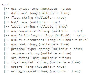
You can also now check out the schema of our DataFrame using the following code.
df.printSchema()
Build a temporary table
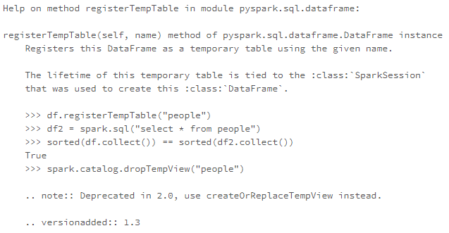
We can leverage the registerTempTable() function to build a temporary table to run SQL commands on our DataFrame at scale! A point to remember is that the lifetime of this temp table is tied to the session. It creates an in-memory table that is scoped to the cluster in which it was created. The data is stored using Hive's highly optimized, in-memory columnar format.
You can also check out saveAsTable(), which creates a permanent, physical table stored in S3 using the Parquet format. This table is accessible to all clusters. The table metadata, including the location of the file(s), is stored within the Hive metastore.
help(df.registerTempTable)
df.registerTempTable("connections")Execute SQL at Scale
Let's look at a few examples of how we can run SQL queries on our table based off of our dataframe. We will start with some simple queries and then look at aggregations, filters, sorting, sub-queries, and pivots in this tutorial.
Connections based on the protocol type
Let's look at how we can get the total number of connections based on the type of connectivity protocol. First, we will get this information using normal DataFrame DSL syntax to perform aggregations.
display(df.groupBy('protocol_type')
          .count()
          .orderBy('count', ascending=False))

Can we also use SQL to perform the same aggregation? Yes, we can leverage the table we built earlier for this!
protocols = sqlContext.sql("""
                           SELECT protocol_type, count(*) as freq
                           FROM connections
                           GROUP BY protocol_type
                           ORDER BY 2 DESC
                           """)
display(protocols)

You can clearly see that you get the same results and don't need to worry about your background infrastructure or how the code is executed. Just write simple SQL!
Connections based on good or bad (attack types) signatures
We will now run a simple aggregation to check the total number of connections based on good (normal) or bad (intrusion attacks) types.
labels = sqlContext.sql("""
                           SELECT label, count(*) as freq
                           FROM connections
                           GROUP BY label
                           ORDER BY 2 DESC
                           """)
display(labels)

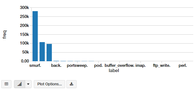
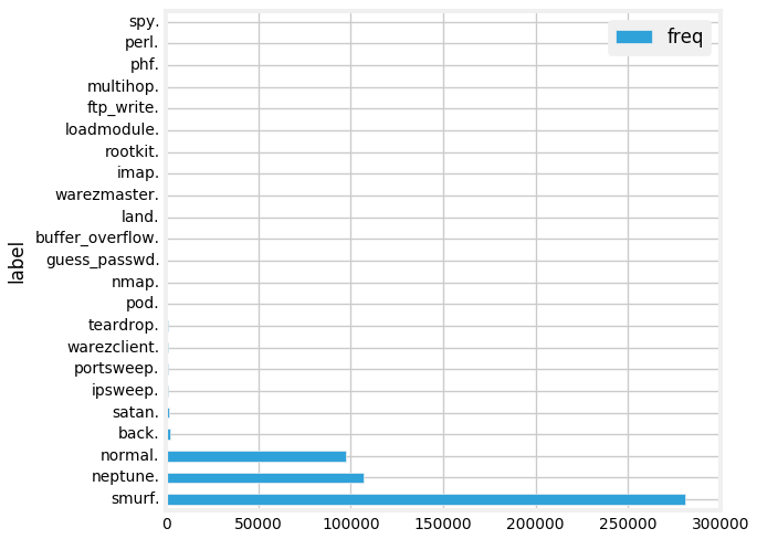
We have a lot of different attack types. We can visualize this in the form of a bar chart. The simplest way is to use the excellent interface options in the Databricks notebook.

This gives us a nice-looking bar chart, which you can customize further by clicking on Plot Options.
Another way is to write the code to do it. You can extract the aggregated data as a Pandas DataFrame and plot it as a regular bar chart.
labels_df = pd.DataFrame(labels.toPandas())
labels_df.set_index("label", drop=True,inplace=True)
labels_fig = labels_df.plot(kind='barh')

plt.rcParams["figure.figsize"] = (7, 5)
plt.rcParams.update({'font.size': 10})
plt.tight_layout()
display(labels_fig.figure)
Connections based on protocols and attacks
Let's look at which protocols are most vulnerable to attacks by using the following SQL query.
attack_protocol = sqlContext.sql("""
                           SELECT
                             protocol_type,
                             CASE label
                               WHEN 'normal.' THEN 'no attack'
                               ELSE 'attack'
                             END AS state,
                             COUNT(*) as freq
                           FROM connections
                           GROUP BY protocol_type, state
                           ORDER BY 3 DESC
                           """)
display(attack_protocol)

Well, it looks like ICMP connections, followed by TCP connections have had the most attacks.
Connection stats based on protocols and attacks
Let's take a look at some statistical measures pertaining to these protocols and attacks for our connection requests.
attack_stats = sqlContext.sql("""
                           SELECT
                             protocol_type,
                             CASE label
                               WHEN 'normal.' THEN 'no attack'
                               ELSE 'attack'
                             END AS state,
                             COUNT(*) as total_freq,
                             ROUND(AVG(src_bytes), 2) as mean_src_bytes,
                             ROUND(AVG(dst_bytes), 2) as mean_dst_bytes,
                             ROUND(AVG(duration), 2) as mean_duration,
                             SUM(num_failed_logins) as total_failed_logins,
                             SUM(num_compromised) as total_compromised,
                             SUM(num_file_creations) as total_file_creations,
                             SUM(su_attempted) as total_root_attempts,
                             SUM(num_root) as total_root_acceses
                           FROM connections
                           GROUP BY protocol_type, state
                           ORDER BY 3 DESC
                           """)
display(attack_stats)

Looks like the average amount of data being transmitted in TCP requests is much higher, which is not surprising. Interestingly, attacks have a much higher average payload of data being transmitted from the source to the destination.
Filtering connection stats based on the TCP protocol by service and attack type
Let's take a closer look at TCP attacks, given that we have more relevant data and statistics for the same. We will now aggregate different types of TCP attacks based on service and attack type and observe different metrics.
tcp_attack_stats = sqlContext.sql("""
                                   SELECT
                                     service,
                                     label as attack_type,
                                     COUNT(*) as total_freq,
                                     ROUND(AVG(duration), 2) as mean_duration,
                                     SUM(num_failed_logins) as total_failed_logins,
                                     SUM(num_file_creations) as total_file_creations,
                                     SUM(su_attempted) as total_root_attempts,
                                     SUM(num_root) as total_root_acceses
                                   FROM connections
                                   WHERE protocol_type = 'tcp'
                                   AND label != 'normal.'
                                   GROUP BY service, attack_type
                                   ORDER BY total_freq DESC
                                   """)
display(tcp_attack_stats)

There are a lot of attack types, and the preceding output shows a specific section of them.
Filtering connection stats based on the TCP protocol by service and attack type
We will now filter some of these attack types by imposing some constraints in our query based on duration, file creations, and root accesses.
tcp_attack_stats = sqlContext.sql("""
                                   SELECT
                                     service,
                                     label as attack_type,
                                     COUNT(*) as total_freq,
                                     ROUND(AVG(duration), 2) as mean_duration,
                                     SUM(num_failed_logins) as total_failed_logins,
                                     SUM(num_file_creations) as total_file_creations,
                                     SUM(su_attempted) as total_root_attempts,
                                     SUM(num_root) as total_root_acceses
                                   FROM connections
                                   WHERE (protocol_type = 'tcp'
                                          AND label != 'normal.')
                                   GROUP BY service, attack_type
                                   HAVING (mean_duration >= 50
                                           AND total_file_creations >= 5
                                           AND total_root_acceses >= 1)
                                   ORDER BY total_freq DESC
                                   """)
display(tcp_attack_stats)

It's interesting to see that multi-hop attacks can get root accesses to the destination hosts!
Subqueries to filter TCP attack types based on service
Let's try to get all the TCP attacks based on service and attack type such that the overall mean duration of these attacks is greater than zero (> 0). For this, we can do an inner query with all aggregation statistics and extract the relevant queries and apply a mean duration filter in the outer query, as shown below.
tcp_attack_stats = sqlContext.sql("""
                                   SELECT
                                     t.service,
                                     t.attack_type,
                                     t.total_freq
                                   FROM
                                   (SELECT
                                     service,
                                     label as attack_type,
                                     COUNT(*) as total_freq,
                                     ROUND(AVG(duration), 2) as mean_duration,
                                     SUM(num_failed_logins) as total_failed_logins,
                                     SUM(num_file_creations) as total_file_creations,
                                     SUM(su_attempted) as total_root_attempts,
                                     SUM(num_root) as total_root_acceses
                                   FROM connections
                                   WHERE protocol_type = 'tcp'
                                   AND label != 'normal.'
                                   GROUP BY service, attack_type
                                   ORDER BY total_freq DESC) as t
                                     WHERE t.mean_duration > 0
                                   """)
display(tcp_attack_stats)

This is nice! Now another interesting way to view this data is to use a pivot table, where one attribute represents rows and another one represents columns. Let's see if we can leverage Spark DataFrames to do this!
Build a pivot table from aggregated data
We will build upon the previous DataFrame object where we aggregated attacks based on type and service. For this, we can leverage the power of Spark DataFrames and the DataFrame DSL.
display((tcp_attack_stats.groupby('service')
                         .pivot('attack_type')
                         .agg({'total_freq':'max'})
                         .na.fill(0))
)

We get a nice, neat pivot table showing all the occurrences based on service and attack type!
Next steps
I would encourage you to go out and play with Spark SQL and DataFrames. You can even import my notebook and play with it in your own account.
Feel free to refer to my GitHub repository also for all the code and notebooks used in this article. It covers things we didn't cover here, including:
- Joins
- Window functions
- Detailed operations and transformations of Spark DataFrames
You can also access my tutorial as a Jupyter Notebook, in case you want to use it offline.
There are plenty of articles and tutorials available online, so I recommend you check them out. One useful resource is Databricks' complete guide to Spark SQL.
Thinking of working with JSON data but unsure of using Spark SQL? Databricks supports it! Check out this excellent guide to JSON support in Spark SQL.
Interested in advanced concepts like window functions and ranks in SQL? Take a look at "Introducing Window Functions in Spark SQL."
I will write another article covering some of these concepts in an intuitive way, which should be easy for you to understand. Stay tuned!
In case you have any feedback or queries, you can reach out to me on LinkedIn.
This article originally appeared on Medium's Towards Data Science channel and is republished with permission.


1 Comment