Detecting malaria with deep learning

Artificial intelligence (AI) and open source tools, technologies, and frameworks are a powerful combination for improving society. "Health is wealth" is perhaps a cliche, yet it's very accurate! In this article, we will examine how AI can be leveraged for detecting the deadly disease malaria with a low-cost, effective, and accurate open source deep learning solution.

While I am neither a doctor nor a healthcare researcher and I'm nowhere near as qualified as they are, I am interested in applying AI to healthcare research. My intent in this article is to showcase how AI and open source solutions can help malaria detection and reduce manual labor.

Image by:

^{Python and TensorFlow—A great combo to build open source deep learning solutions}

Thanks to the power of Python and deep learning frameworks like TensorFlow, we can build robust, scalable, and effective deep learning solutions. Because these tools are free and open source, we can build solutions that are very cost-effective and easily adopted and used by anyone. Let's get started!

Motivation for the project

Malaria is a deadly, infectious, mosquito-borne disease caused by Plasmodium parasites that are transmitted by the bites of infected female Anopheles mosquitoes. There are five parasites that cause malaria, but two types—P. falciparum and P. vivax—cause the majority of the cases.

Image by:

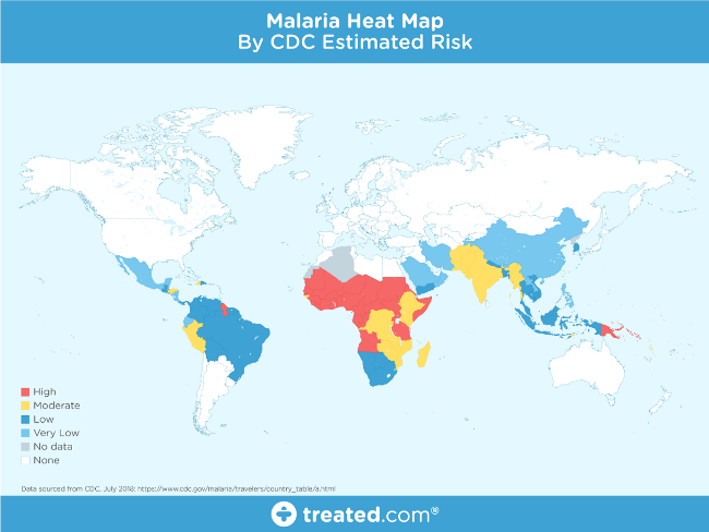
Image from Treated.com

This map shows that malaria is prevalent around the globe, especially in tropical regions, but the nature and fatality of the disease is the primary motivation for this project.

If an infected mosquito bites you, parasites carried by the mosquito enter your blood and start destroying oxygen-carrying red blood cells (RBC). Typically, the first symptoms of malaria are similar to a virus like the flu and they usually begin within a few days or weeks after the mosquito bite. However, these deadly parasites can live in your body for over a year without causing symptoms, and a delay in treatment can lead to complications and even death. Therefore, early detection can save lives.

The World Health Organization's (WHO) malaria facts indicate that nearly half the world's population is at risk from malaria, and there are over 200 million malaria cases and approximately 400,000 deaths due to malaria every year. This is a motivatation to make malaria detection and diagnosis fast, easy, and effective.

Methods of malaria detection

There are several methods that can be used for malaria detection and diagnosis. The paper on which our project is based, "Pre-trained convolutional neural networks as feature extractors toward improved Malaria parasite detection in thin blood smear images," by Rajaraman, et al., introduces some of the methods, including polymerase chain reaction (PCR) and rapid diagnostic tests (RDT). These two tests are typically used where high-quality microscopy services are not readily available.

The standard malaria diagnosis is typically based on a blood-smear workflow, according to Carlos Ariza's article "Malaria Hero: A web app for faster malaria diagnosis," which I learned about in Adrian Rosebrock's "Deep learning and medical image analysis with Keras." I appreciate the authors of these excellent resources for giving me more perspective on malaria prevalence, diagnosis, and treatment.

Image by:

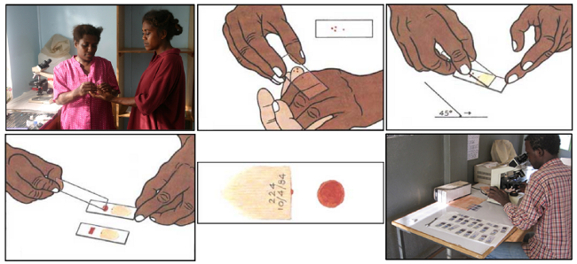
^{A blood smear workflow for Malaria detection.}

According to WHO protocol, diagnosis typically involves intensive examination of the blood smear at 100X magnification. Trained people manually count how many red blood cells contain parasites out of 5,000 cells. As the Rajaraman, et al., paper cited above explains:

Thick blood smears assist in detecting the presence of parasites while thin blood smears assist in identifying the species of the parasite causing the infection (Centers for Disease Control and Prevention, 2012). The diagnostic accuracy heavily depends on human expertise and can be adversely impacted by the inter-observer variability and the liability imposed by large-scale diagnoses in disease-endemic/resource-constrained regions (Mitiku, Mengistu, and Gelaw, 2003). Alternative techniques such as polymerase chain reaction (PCR) and rapid diagnostic tests (RDT) are used; however, PCR analysis is limited in its performance (Hommelsheim, et al., 2014) and RDTs are less cost-effective in disease-endemic regions (Hawkes, Katsuva, and Masumbuko, 2009).

Thus, malaria detection could benefit from automation using deep learning.

Deep learning for malaria detection

Manual diagnosis of blood smears is an intensive manual process that requires expertise in classifying and counting parasitized and uninfected cells. This process may not scale well, especially in regions where the right expertise is hard to find. Some advancements have been made in leveraging state-of-the-art image processing and analysis techniques to extract hand-engineered features and build machine learning-based classification models. However, these models are not scalable with more data being available for training and given the fact that hand-engineered features take a lot of time.

Deep learning models, or more specifically convolutional neural networks (CNNs), have proven very effective in a wide variety of computer vision tasks. (If you would like additional background knowledge on CNNs, I recommend reading CS231n Convolutional Neural Networks for Visual Recognition.) Briefly, the key layers in a CNN model include convolution and pooling layers, as shown in the following figure.

Image by:

^{A typical CNN architecture.}

Convolution layers learn spatial hierarchical patterns from data, which are also translation-invariant, so they are able to learn different aspects of images. For example, the first convolution layer will learn small and local patterns, such as edges and corners, a second convolution layer will learn larger patterns based on the features from the first layers, and so on. This allows CNNs to automate feature engineering and learn effective features that generalize well on new data points. Pooling layers helps with downsampling and dimension reduction.

Thus, CNNs help with automated and scalable feature engineering. Also, plugging in dense layers at the end of the model enables us to perform tasks like image classification. Automated malaria detection using deep learning models like CNNs could be very effective, cheap, and scalable, especially with the advent of transfer learning and pre-trained models that work quite well, even with constraints like less data.

The Rajaraman, et al., paper leverages six pre-trained models on a dataset to obtain an impressive accuracy of 95.9% in detecting malaria vs. non-infected samples. Our focus is to try some simple CNN models from scratch and a couple of pre-trained models using transfer learning to see the results we can get on the same dataset. We will use open source tools and frameworks, including Python and TensorFlow, to build our models.

The dataset

The data for our analysis comes from researchers at the Lister Hill National Center for Biomedical Communications (LHNCBC), part of the National Library of Medicine (NLM), who have carefully collected and annotated the publicly available dataset of healthy and infected blood smear images. These researchers have developed a mobile application for malaria detection that runs on a standard Android smartphone attached to a conventional light microscope. They used Giemsa-stained thin blood smear slides from 150 P. falciparum-infected and 50 healthy patients, collected and photographed at Chittagong Medical College Hospital, Bangladesh. The smartphone's built-in camera acquired images of slides for each microscopic field of view. The images were manually annotated by an expert slide reader at the Mahidol-Oxford Tropical Medicine Research Unit in Bangkok, Thailand.

Let's briefly check out the dataset's structure. First, I will install some basic dependencies (based on the operating system being used).

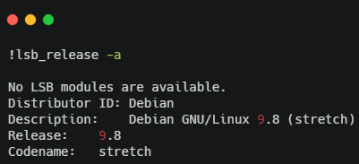
I am using a Debian-based system on the cloud with a GPU so I can run my models faster. To view the directory structure, we must install the tree dependency (if we don't have it) using sudo apt install tree.

We have two folders that contain images of cells, infected and healthy. We can get further details about the total number of images by entering:

import os
import glob

base_dir = os.path.join('./cell_images')
infected_dir = os.path.join(base_dir,'Parasitized')
healthy_dir = os.path.join(base_dir,'Uninfected')

infected_files = glob.glob(infected_dir+'/*.png')
healthy_files = glob.glob(healthy_dir+'/*.png')
len(infected_files), len(healthy_files)

# Output
(13779, 13779)

It looks like we have a balanced dataset with 13,779 malaria and 13,779 non-malaria (uninfected) cell images. Let's build a data frame from this, which we will use when we start building our datasets.

import numpy as np
import pandas as pd

np.random.seed(42)

files_df = pd.DataFrame({
    'filename': infected_files + healthy_files,
    'label': ['malaria'] * len(infected_files) + ['healthy'] * len(healthy_files)
}).sample(frac=1, random_state=42).reset_index(drop=True)

files_df.head()

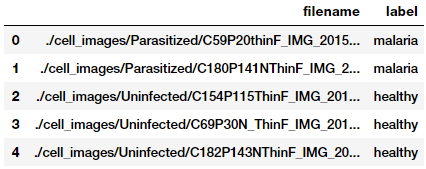
Build and explore image datasets

To build deep learning models, we need training data, but we also need to test the model's performance on unseen data. We will use a 60:10:30 split for train, validation, and test datasets, respectively. We will leverage the train and validation datasets during training and check the performance of the model on the test dataset.

from sklearn.model_selection import train_test_split
from collections import Counter

train_files, test_files, train_labels, test_labels = train_test_split(files_df['filename'].values,
                                                                      files_df['label'].values, 
                                                                      test_size=0.3, random_state=42)
train_files, val_files, train_labels, val_labels = train_test_split(train_files,
                                                                    train_labels, 
                                                                    test_size=0.1, random_state=42)

print(train_files.shape, val_files.shape, test_files.shape)
print('Train:', Counter(train_labels), '\nVal:', Counter(val_labels), '\nTest:', Counter(test_labels))

# Output
(17361,) (1929,) (8268,)
Train: Counter({'healthy': 8734, 'malaria': 8627}) 
Val: Counter({'healthy': 970, 'malaria': 959}) 
Test: Counter({'malaria': 4193, 'healthy': 4075})

The images will not be of equal dimensions because blood smears and cell images vary based on the human, the test method, and the orientation of the photo. Let's get some summary statistics of our training dataset to determine the optimal image dimensions (remember, we don't touch the test dataset at all!).

import cv2
from concurrent import futures
import threading

def get_img_shape_parallel(idx, img, total_imgs):
    if idx % 5000 == 0 or idx == (total_imgs - 1):
        print('{}: working on img num: {}'.format(threading.current_thread().name,
                                                  idx))
    return cv2.imread(img).shape
  
ex = futures.ThreadPoolExecutor(max_workers=None)
data_inp = [(idx, img, len(train_files)) for idx, img in enumerate(train_files)]
print('Starting Img shape computation:')
train_img_dims_map = ex.map(get_img_shape_parallel, 
                            [record[0] for record in data_inp],
                            [record[1] for record in data_inp],
                            [record[2] for record in data_inp])
train_img_dims = list(train_img_dims_map)
print('Min Dimensions:', np.min(train_img_dims, axis=0)) 
print('Avg Dimensions:', np.mean(train_img_dims, axis=0))
print('Median Dimensions:', np.median(train_img_dims, axis=0))
print('Max Dimensions:', np.max(train_img_dims, axis=0))


# Output
Starting Img shape computation:
ThreadPoolExecutor-0_0: working on img num: 0
ThreadPoolExecutor-0_17: working on img num: 5000
ThreadPoolExecutor-0_15: working on img num: 10000
ThreadPoolExecutor-0_1: working on img num: 15000
ThreadPoolExecutor-0_7: working on img num: 17360
Min Dimensions: [46 46  3]
Avg Dimensions: [132.77311215 132.45757733   3.]
Median Dimensions: [130. 130.   3.]
Max Dimensions: [385 394   3]

We apply parallel processing to speed up the image-read operations and, based on the summary statistics, we will resize each image to 125x125 pixels. Let's load up all of our images and resize them to these fixed dimensions.

IMG_DIMS = (125, 125)

def get_img_data_parallel(idx, img, total_imgs):
    if idx % 5000 == 0 or idx == (total_imgs - 1):
        print('{}: working on img num: {}'.format(threading.current_thread().name,
                                                  idx))
    img = cv2.imread(img)
    img = cv2.resize(img, dsize=IMG_DIMS, 
                     interpolation=cv2.INTER_CUBIC)
    img = np.array(img, dtype=np.float32)
    return img

ex = futures.ThreadPoolExecutor(max_workers=None)
train_data_inp = [(idx, img, len(train_files)) for idx, img in enumerate(train_files)]
val_data_inp = [(idx, img, len(val_files)) for idx, img in enumerate(val_files)]
test_data_inp = [(idx, img, len(test_files)) for idx, img in enumerate(test_files)]

print('Loading Train Images:')
train_data_map = ex.map(get_img_data_parallel, 
                        [record[0] for record in train_data_inp],
                        [record[1] for record in train_data_inp],
                        [record[2] for record in train_data_inp])
train_data = np.array(list(train_data_map))

print('\nLoading Validation Images:')
val_data_map = ex.map(get_img_data_parallel, 
                        [record[0] for record in val_data_inp],
                        [record[1] for record in val_data_inp],
                        [record[2] for record in val_data_inp])
val_data = np.array(list(val_data_map))

print('\nLoading Test Images:')
test_data_map = ex.map(get_img_data_parallel, 
                        [record[0] for record in test_data_inp],
                        [record[1] for record in test_data_inp],
                        [record[2] for record in test_data_inp])
test_data = np.array(list(test_data_map))

train_data.shape, val_data.shape, test_data.shape  


# Output
Loading Train Images:
ThreadPoolExecutor-1_0: working on img num: 0
ThreadPoolExecutor-1_12: working on img num: 5000
ThreadPoolExecutor-1_6: working on img num: 10000
ThreadPoolExecutor-1_10: working on img num: 15000
ThreadPoolExecutor-1_3: working on img num: 17360

Loading Validation Images:
ThreadPoolExecutor-1_13: working on img num: 0
ThreadPoolExecutor-1_18: working on img num: 1928

Loading Test Images:
ThreadPoolExecutor-1_5: working on img num: 0
ThreadPoolExecutor-1_19: working on img num: 5000
ThreadPoolExecutor-1_8: working on img num: 8267
((17361, 125, 125, 3), (1929, 125, 125, 3), (8268, 125, 125, 3))

We leverage parallel processing again to speed up computations pertaining to image load and resizing. Finally, we get our image tensors of the desired dimensions, as depicted in the preceding output. We can now view some sample cell images to get an idea of how our data looks.

import matplotlib.pyplot as plt
%matplotlib inline

plt.figure(1 , figsize = (8 , 8))
n = 0 
for i in range(16):
    n += 1 
    r = np.random.randint(0 , train_data.shape[0] , 1)
    plt.subplot(4 , 4 , n)
    plt.subplots_adjust(hspace = 0.5 , wspace = 0.5)
    plt.imshow(train_data[r[0]]/255.)
    plt.title('{}'.format(train_labels[r[0]]))
    plt.xticks([]) , plt.yticks([])

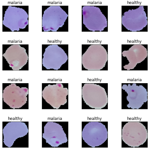
Based on these sample images, we can see some subtle differences between malaria and healthy cell images. We will make our deep learning models try to learn these patterns during model training.

Before can we start training our models, we must set up some basic configuration settings.

BATCH_SIZE = 64
NUM_CLASSES = 2
EPOCHS = 25
INPUT_SHAPE = (125, 125, 3)

train_imgs_scaled = train_data / 255.
val_imgs_scaled = val_data / 255.

# encode text category labels
from sklearn.preprocessing import LabelEncoder

le = LabelEncoder()
le.fit(train_labels)
train_labels_enc = le.transform(train_labels)
val_labels_enc = le.transform(val_labels)

print(train_labels[:6], train_labels_enc[:6])


# Output
['malaria' 'malaria' 'malaria' 'healthy' 'healthy' 'malaria'] [1 1 1 0 0 1]

We fix our image dimensions, batch size, and epochs and encode our categorical class labels. The alpha version of TensorFlow 2.0 was released in March 2019, and this exercise is the perfect excuse to try it out.

import tensorflow as tf

# Load the TensorBoard notebook extension (optional)
%load_ext tensorboard.notebook

tf.random.set_seed(42)
tf.__version__

# Output
'2.0.0-alpha0'

Deep learning model training

In the model training phase, we will build three deep learning models, train them with our training data, and compare their performance using the validation data. We will then save these models and use them later in the model evaluation phase.

Model 1: CNN from scratch

Our first malaria detection model will build and train a basic CNN from scratch. First, let's define our model architecture.

inp = tf.keras.layers.Input(shape=INPUT_SHAPE)

conv1 = tf.keras.layers.Conv2D(32, kernel_size=(3, 3), 
                               activation='relu', padding='same')(inp)
pool1 = tf.keras.layers.MaxPooling2D(pool_size=(2, 2))(conv1)
conv2 = tf.keras.layers.Conv2D(64, kernel_size=(3, 3), 
                               activation='relu', padding='same')(pool1)
pool2 = tf.keras.layers.MaxPooling2D(pool_size=(2, 2))(conv2)
conv3 = tf.keras.layers.Conv2D(128, kernel_size=(3, 3), 
                               activation='relu', padding='same')(pool2)
pool3 = tf.keras.layers.MaxPooling2D(pool_size=(2, 2))(conv3)

flat = tf.keras.layers.Flatten()(pool3)

hidden1 = tf.keras.layers.Dense(512, activation='relu')(flat)
drop1 = tf.keras.layers.Dropout(rate=0.3)(hidden1)
hidden2 = tf.keras.layers.Dense(512, activation='relu')(drop1)
drop2 = tf.keras.layers.Dropout(rate=0.3)(hidden2)

out = tf.keras.layers.Dense(1, activation='sigmoid')(drop2)

model = tf.keras.Model(inputs=inp, outputs=out)
model.compile(optimizer='adam',
                loss='binary_crossentropy',
                metrics=['accuracy'])
model.summary()


# Output
Model: "model"
_________________________________________________________________
Layer (type)                 Output Shape              Param #   
=================================================================
input_1 (InputLayer)         [(None, 125, 125, 3)]     0         
_________________________________________________________________
conv2d (Conv2D)              (None, 125, 125, 32)      896       
_________________________________________________________________
max_pooling2d (MaxPooling2D) (None, 62, 62, 32)        0         
_________________________________________________________________
conv2d_1 (Conv2D)            (None, 62, 62, 64)        18496     
_________________________________________________________________
...
...
_________________________________________________________________
dense_1 (Dense)              (None, 512)               262656    
_________________________________________________________________
dropout_1 (Dropout)          (None, 512)               0         
_________________________________________________________________
dense_2 (Dense)              (None, 1)                 513       
=================================================================
Total params: 15,102,529
Trainable params: 15,102,529
Non-trainable params: 0
_________________________________________________________________

Based on the architecture in this code, our CNN model has three convolution and pooling layers, followed by two dense layers, and dropouts for regularization. Let's train our model.

import datetime

logdir = os.path.join('/home/dipanzan_sarkar/projects/tensorboard_logs', 
                      datetime.datetime.now().strftime("%Y%m%d-%H%M%S"))
tensorboard_callback = tf.keras.callbacks.TensorBoard(logdir, histogram_freq=1)
reduce_lr = tf.keras.callbacks.ReduceLROnPlateau(monitor='val_loss', factor=0.5,
                              patience=2, min_lr=0.000001)
callbacks = [reduce_lr, tensorboard_callback]

history = model.fit(x=train_imgs_scaled, y=train_labels_enc, 
                    batch_size=BATCH_SIZE,
                    epochs=EPOCHS, 
                    validation_data=(val_imgs_scaled, val_labels_enc), 
                    callbacks=callbacks,
                    verbose=1)
                    

# Output
Train on 17361 samples, validate on 1929 samples
Epoch 1/25
17361/17361 [====] - 32s 2ms/sample - loss: 0.4373 - accuracy: 0.7814 - val_loss: 0.1834 - val_accuracy: 0.9393
Epoch 2/25
17361/17361 [====] - 30s 2ms/sample - loss: 0.1725 - accuracy: 0.9434 - val_loss: 0.1567 - val_accuracy: 0.9513
...
...
Epoch 24/25
17361/17361 [====] - 30s 2ms/sample - loss: 0.0036 - accuracy: 0.9993 - val_loss: 0.3693 - val_accuracy: 0.9565
Epoch 25/25
17361/17361 [====] - 30s 2ms/sample - loss: 0.0034 - accuracy: 0.9994 - val_loss: 0.3699 - val_accuracy: 0.9559
                    
      

We get a validation accuracy of 95.6%, which is pretty good, although our model looks to be overfitting slightly (based on looking at our training accuracy, which is 99.9%). We can get a clear perspective on this by plotting the training and validation accuracy and loss curves.

f, (ax1, ax2) = plt.subplots(1, 2, figsize=(12, 4))
t = f.suptitle('Basic CNN Performance', fontsize=12)
f.subplots_adjust(top=0.85, wspace=0.3)

max_epoch = len(history.history['accuracy'])+1
epoch_list = list(range(1,max_epoch))
ax1.plot(epoch_list, history.history['accuracy'], label='Train Accuracy')
ax1.plot(epoch_list, history.history['val_accuracy'], label='Validation Accuracy')
ax1.set_xticks(np.arange(1, max_epoch, 5))
ax1.set_ylabel('Accuracy Value')
ax1.set_xlabel('Epoch')
ax1.set_title('Accuracy')
l1 = ax1.legend(loc="best")

ax2.plot(epoch_list, history.history['loss'], label='Train Loss')
ax2.plot(epoch_list, history.history['val_loss'], label='Validation Loss')
ax2.set_xticks(np.arange(1, max_epoch, 5))
ax2.set_ylabel('Loss Value')
ax2.set_xlabel('Epoch')
ax2.set_title('Loss')
l2 = ax2.legend(loc="best")

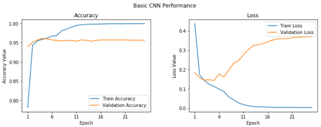
We can see after the fifth epoch that things don't seem to improve a whole lot overall. Let's save this model for future evaluation.

model.save('basic_cnn.h5')

Deep transfer learning

Just like humans have an inherent capability to transfer knowledge across tasks, transfer learning enables us to utilize knowledge from previously learned tasks and apply it to newer, related ones, even in the context of machine learning or deep learning. If you are interested in doing a deep-dive on transfer learning, you can read my article "A comprehensive hands-on guide to transfer learning with real-world applications in deep learning" and my book Hands-On Transfer Learning with Python.

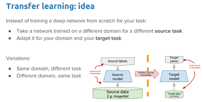
The idea we want to explore in this exercise is:

Can we leverage a pre-trained deep learning model (which was trained on a large dataset, like ImageNet) to solve the problem of malaria detection by applying and transferring its knowledge in the context of our problem?

We will apply the two most popular strategies for deep transfer learning.

• Pre-trained model as a feature extractor
• Pre-trained model with fine-tuning

We will be using the pre-trained VGG-19 deep learning model, developed by the Visual Geometry Group (VGG) at the University of Oxford, for our experiments. A pre-trained model like VGG-19 is trained on a huge dataset (ImageNet) with a lot of diverse image categories. Therefore, the model should have learned a robust hierarchy of features, which are spatial-, rotational-, and translation-invariant with regard to features learned by CNN models. Hence, the model, having learned a good representation of features for over a million images, can act as a good feature extractor for new images suitable for computer vision problems like malaria detection. Let's discuss the VGG-19 model architecture before unleashing the power of transfer learning on our problem.

Understanding the VGG-19 model

The VGG-19 model is a 19-layer (convolution and fully connected) deep learning network built on the ImageNet database, which was developed for the purpose of image recognition and classification. This model was built by Karen Simonyan and Andrew Zisserman and is described in their paper "Very deep convolutional networks for large-scale image recognition." The architecture of the VGG-19 model is:

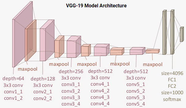
You can see that we have a total of 16 convolution layers using 3x3 convolution filters along with max pooling layers for downsampling and two fully connected hidden layers of 4,096 units in each layer followed by a dense layer of 1,000 units, where each unit represents one of the image categories in the ImageNet database. We do not need the last three layers since we will be using our own fully connected dense layers to predict malaria. We are more concerned with the first five blocks so we can leverage the VGG model as an effective feature extractor.

We will use one of the models as a simple feature extractor by freezing the five convolution blocks to make sure their weights aren't updated after each epoch. For the last model, we will apply fine-tuning to the VGG model, where we will unfreeze the last two blocks (Block 4 and Block 5) so that their weights will be updated in each epoch (per batch of data) as we train our own model.

Model 2: Pre-trained model as a feature extractor

For building this model, we will leverage TensorFlow to load up the VGG-19 model and freeze the convolution blocks so we can use them as an image feature extractor. We will plug in our own dense layers at the end to perform the classification task.

vgg = tf.keras.applications.vgg19.VGG19(include_top=False, weights='imagenet', 
                                        input_shape=INPUT_SHAPE)
vgg.trainable = False
# Freeze the layers
for layer in vgg.layers:
    layer.trainable = False
    
base_vgg = vgg
base_out = base_vgg.output
pool_out = tf.keras.layers.Flatten()(base_out)
hidden1 = tf.keras.layers.Dense(512, activation='relu')(pool_out)
drop1 = tf.keras.layers.Dropout(rate=0.3)(hidden1)
hidden2 = tf.keras.layers.Dense(512, activation='relu')(drop1)
drop2 = tf.keras.layers.Dropout(rate=0.3)(hidden2)

out = tf.keras.layers.Dense(1, activation='sigmoid')(drop2)

model = tf.keras.Model(inputs=base_vgg.input, outputs=out)
model.compile(optimizer=tf.keras.optimizers.RMSprop(lr=1e-4),
                loss='binary_crossentropy',
                metrics=['accuracy'])
model.summary()


# Output
Model: "model_1"
_________________________________________________________________
Layer (type)                 Output Shape              Param #   
=================================================================
input_2 (InputLayer)         [(None, 125, 125, 3)]     0         
_________________________________________________________________
block1_conv1 (Conv2D)        (None, 125, 125, 64)      1792      
_________________________________________________________________
block1_conv2 (Conv2D)        (None, 125, 125, 64)      36928     
_________________________________________________________________
...
...
_________________________________________________________________
block5_pool (MaxPooling2D)   (None, 3, 3, 512)         0         
_________________________________________________________________
flatten_1 (Flatten)          (None, 4608)              0         
_________________________________________________________________
dense_3 (Dense)              (None, 512)               2359808   
_________________________________________________________________
dropout_2 (Dropout)          (None, 512)               0         
_________________________________________________________________
dense_4 (Dense)              (None, 512)               262656    
_________________________________________________________________
dropout_3 (Dropout)          (None, 512)               0         
_________________________________________________________________
dense_5 (Dense)              (None, 1)                 513       
=================================================================
Total params: 22,647,361
Trainable params: 2,622,977
Non-trainable params: 20,024,384
_________________________________________________________________

It is evident from this output that we have a lot of layers in our model and we will be using the frozen layers of the VGG-19 model as feature extractors only. You can use the following code to verify how many layers in our model are indeed trainable and how many total layers are present in our network.

print("Total Layers:", len(model.layers))
print("Total trainable layers:", 
      sum([1 for l in model.layers if l.trainable]))

# Output
Total Layers: 28
Total trainable layers: 6

We will now train our model using similar configurations and callbacks to the ones we used in our previous model. Refer to my GitHub repository for the complete code to train the model. We observe the following plots showing the model's accuracy and loss.

Image by:

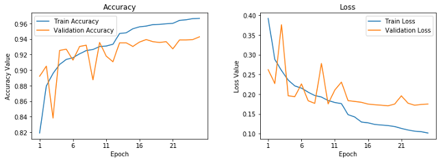
^{Learning curves for frozen pre-trained CNN.}

This shows that our model is not overfitting as much as our basic CNN model, but the performance is slightly less than our basic CNN model. Let's save this model for future evaluation.

model.save('vgg_frozen.h5')

Model 3: Fine-tuned pre-trained model with image augmentation

In our final model, we will fine-tune the weights of the layers in the last two blocks of our pre-trained VGG-19 model. We will also introduce the concept of image augmentation. The idea behind image augmentation is exactly as the name sounds. We load in existing images from our training dataset and apply some image transformation operations to them, such as rotation, shearing, translation, zooming, and so on, to produce new, altered versions of existing images. Due to these random transformations, we don't get the same images each time. We will leverage an excellent utility called ImageDataGenerator in tf.keras that can help build image augmentors.

train_datagen = tf.keras.preprocessing.image.ImageDataGenerator(rescale=1./255,
                                                                zoom_range=0.05, 
                                                                rotation_range=25,
                                                                width_shift_range=0.05, 
                                                                height_shift_range=0.05, 
                                                                shear_range=0.05, horizontal_flip=True, 
                                                                fill_mode='nearest')

val_datagen = tf.keras.preprocessing.image.ImageDataGenerator(rescale=1./255)

# build image augmentation generators
train_generator = train_datagen.flow(train_data, train_labels_enc, batch_size=BATCH_SIZE, shuffle=True)
val_generator = val_datagen.flow(val_data, val_labels_enc, batch_size=BATCH_SIZE, shuffle=False)

We will not apply any transformations on our validation dataset (except for scaling the images, which is mandatory) since we will be using it to evaluate our model performance per epoch. For a detailed explanation of image augmentation in the context of transfer learning, feel free to check out my article cited above. Let's look at some sample results from a batch of image augmentation transforms.

img_id = 0
sample_generator = train_datagen.flow(train_data[img_id:img_id+1], train_labels[img_id:img_id+1],
                                      batch_size=1)
sample = [next(sample_generator) for i in range(0,5)]
fig, ax = plt.subplots(1,5, figsize=(16, 6))
print('Labels:', [item[1][0] for item in sample])
l = [ax[i].imshow(sample[i][0][0]) for i in range(0,5)]

You can clearly see the slight variations of our images in the preceding output. We will now build our deep learning model, making sure the last two blocks of the VGG-19 model are trainable.

vgg = tf.keras.applications.vgg19.VGG19(include_top=False, weights='imagenet', 
                                        input_shape=INPUT_SHAPE)
# Freeze the layers
vgg.trainable = True

set_trainable = False
for layer in vgg.layers:
    if layer.name in ['block5_conv1', 'block4_conv1']:
        set_trainable = True
    if set_trainable:
        layer.trainable = True
    else:
        layer.trainable = False
    
base_vgg = vgg
base_out = base_vgg.output
pool_out = tf.keras.layers.Flatten()(base_out)
hidden1 = tf.keras.layers.Dense(512, activation='relu')(pool_out)
drop1 = tf.keras.layers.Dropout(rate=0.3)(hidden1)
hidden2 = tf.keras.layers.Dense(512, activation='relu')(drop1)
drop2 = tf.keras.layers.Dropout(rate=0.3)(hidden2)

out = tf.keras.layers.Dense(1, activation='sigmoid')(drop2)

model = tf.keras.Model(inputs=base_vgg.input, outputs=out)
model.compile(optimizer=tf.keras.optimizers.RMSprop(lr=1e-5),
                loss='binary_crossentropy',
                metrics=['accuracy'])

print("Total Layers:", len(model.layers))
print("Total trainable layers:", sum([1 for l in model.layers if l.trainable]))


# Output
Total Layers: 28
Total trainable layers: 16

We reduce the learning rate in our model since we don't want to make to large weight updates to the pre-trained layers when fine-tuning. The model's training process will be slightly different since we are using data generators, so we will be leveraging the fit_generator(…) function.

tensorboard_callback = tf.keras.callbacks.TensorBoard(logdir, histogram_freq=1)
reduce_lr = tf.keras.callbacks.ReduceLROnPlateau(monitor='val_loss', factor=0.5,
                              patience=2, min_lr=0.000001)

callbacks = [reduce_lr, tensorboard_callback]
train_steps_per_epoch = train_generator.n // train_generator.batch_size
val_steps_per_epoch = val_generator.n // val_generator.batch_size
history = model.fit_generator(train_generator, steps_per_epoch=train_steps_per_epoch, epochs=EPOCHS,
                              validation_data=val_generator, validation_steps=val_steps_per_epoch, 
                              verbose=1)


# Output
Epoch 1/25
271/271 [====] - 133s 489ms/step - loss: 0.2267 - accuracy: 0.9117 - val_loss: 0.1414 - val_accuracy: 0.9531
Epoch 2/25
271/271 [====] - 129s 475ms/step - loss: 0.1399 - accuracy: 0.9552 - val_loss: 0.1292 - val_accuracy: 0.9589
...
...
Epoch 24/25
271/271 [====] - 128s 473ms/step - loss: 0.0815 - accuracy: 0.9727 - val_loss: 0.1466 - val_accuracy: 0.9682
Epoch 25/25
271/271 [====] - 128s 473ms/step - loss: 0.0792 - accuracy: 0.9729 - val_loss: 0.1127 - val_accuracy: 0.9641

This looks to be our best model yet. It gives us a validation accuracy of almost 96.5% and, based on the training accuracy, it doesn't look like our model is overfitting as much as our first model. This can be verified with the following learning curves.

Image by:

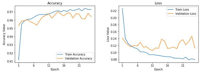
^{Learning curves for fine-tuned pre-trained CNN.}

Let's save this model so we can use it for model evaluation on our test dataset.

model.save('vgg_finetuned.h5')

This completes our model training phase. We are now ready to test the performance of our models on the actual test dataset!

Deep learning model performance evaluation

We will evaluate the three models we built in the training phase by making predictions with them on the data from our test dataset—because just validation is not enough! We have also built a nifty utility module called model_evaluation_utils, which we can use to evaluate the performance of our deep learning models with relevant classification metrics. The first step is to scale our test data.

test_imgs_scaled = test_data / 255.
test_imgs_scaled.shape, test_labels.shape

# Output
((8268, 125, 125, 3), (8268,))

The next step involves loading our saved deep learning models and making predictions on the test data.

# Load Saved Deep Learning Models
basic_cnn = tf.keras.models.load_model('./basic_cnn.h5')
vgg_frz = tf.keras.models.load_model('./vgg_frozen.h5')
vgg_ft = tf.keras.models.load_model('./vgg_finetuned.h5')

# Make Predictions on Test Data
basic_cnn_preds = basic_cnn.predict(test_imgs_scaled, batch_size=512)
vgg_frz_preds = vgg_frz.predict(test_imgs_scaled, batch_size=512)
vgg_ft_preds = vgg_ft.predict(test_imgs_scaled, batch_size=512)

basic_cnn_pred_labels = le.inverse_transform([1 if pred > 0.5 else 0 
                                                  for pred in basic_cnn_preds.ravel()])
vgg_frz_pred_labels = le.inverse_transform([1 if pred > 0.5 else 0 
                                                  for pred in vgg_frz_preds.ravel()])
vgg_ft_pred_labels = le.inverse_transform([1 if pred > 0.5 else 0 
                                                  for pred in vgg_ft_preds.ravel()])

The final step is to leverage our model_evaluation_utils module and check the performance of each model with relevant classification metrics.

import model_evaluation_utils as meu
import pandas as pd

basic_cnn_metrics = meu.get_metrics(true_labels=test_labels, predicted_labels=basic_cnn_pred_labels)
vgg_frz_metrics = meu.get_metrics(true_labels=test_labels, predicted_labels=vgg_frz_pred_labels)
vgg_ft_metrics = meu.get_metrics(true_labels=test_labels, predicted_labels=vgg_ft_pred_labels)

pd.DataFrame([basic_cnn_metrics, vgg_frz_metrics, vgg_ft_metrics], 
             index=['Basic CNN', 'VGG-19 Frozen', 'VGG-19 Fine-tuned'])

It looks like our third model performs best on the test dataset, giving a model accuracy and an F₁-score of 96%, which is pretty good and quite comparable to the more complex models mentioned in the research paper and articles we mentioned earlier.

Conclusion

Malaria detection is not an easy procedure, and the availability of qualified personnel around the globe is a serious concern in the diagnosis and treatment of cases. We looked at an interesting real-world medical imaging case study of malaria detection. Easy-to-build, open source techniques leveraging AI can give us state-of-the-art accuracy in detecting malaria, thus enabling AI for social good.

I encourage you to check out the articles and research papers mentioned in this article, without which it would have been impossible for me to conceptualize and write it. If you are interested in running or adopting these techniques, all the code used in this article is available on my GitHub repository. Remember to download the data from the official website.

Let's hope for more adoption of open source AI capabilities in healthcare to make it less expensive and more accessible for everyone around the world!