JavaScript (also known as JS) is the lingua franca of the web, as it is supported by all the major web browsers—the other languages that run in browsers are transpiled (or translated) to JavaScript. Sometimes JS can be confusing, but I find it pleasant to use because I try to stick to the good parts. JavaScript was created to run in a browser, but it can also be used in other contexts, such as an embedded language or for server-side applications.
In this tutorial, I will explain how to write a program that will run in Node.js, which is a runtime environment that can execute JavaScript applications. What I like the most about Node.js is its event-driven architecture for asynchronous programming. With this approach, functions (aka callbacks) can be attached to certain events; when the attached event occurs, the callback executes. This way, the developer does not have to write a main loop because the runtime takes care of that.
JavaScript also has new async functions that use a different syntax, but I think they hide the event-driven architecture too well to use them in a how-to article. So, in this tutorial, I will use the traditional callbacks approach, even though it is not necessary for this case.
Understanding the program task
The program task in this tutorial is to:
- Read some data from a CSV file that contains the Anscombe's quartet dataset
- Interpolate the data with a straight line (i.e., f(x) = m·x + q)
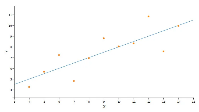
- Plot the result to an image file
For more details about this task, you can read the previous articles in this series, which do the same task in Python and GNU Octave and C and C++. The full source code for all the examples is available in my polyglot_fit repository on GitLab.
Installing
Before you can run this example, you must install Node.js and its package manager npm. To install them on Fedora, run:
$ sudo dnf install nodejs npmOn Ubuntu:
$ sudo apt install nodejs npmNext, use npm to install the required packages. Packages are installed in a local node_modules subdirectory, so Node.js can search for packages in that folder. The required packages are:
- CSV Parse for parsing the CSV file
- Simple Statistics for calculating the data correlation factor
- Regression-js for determining the fitting line
- D3-Node for server-side plotting
Run npm to install the packages:
$ npm install csv-parse simple-statistics regression d3-nodeCommenting code
Just like in C, in JavaScript, you can insert comments by putting // before your comment, and the interpreter will discard the rest of the line. Another option: JavaScript will discard anything between /* and */:
// This is a comment ignored by the interpreter.
/* Also this is ignored */
Loading modules
You can load modules with the require() function. The function returns an object that contains a module's functions:
const EventEmitter = require('events');
const fs = require('fs');
const csv = require('csv-parser');
const regression = require('regression');
const ss = require('simple-statistics');
const D3Node = require('d3-node');
Some of these modules are part of the Node.js standard library, so you do not need to install them with npm.
Defining variables
Variables do not have to be declared before they are used, but if they are used without a declaration, they will be defined as global variables. Generally, global variables are considered bad practice, as they could lead to bugs if they're used carelessly. To declare a variable, you can use the var, let, and const statements. Variables can contain any kind of data (even functions!). You can create some objects by applying the new operator to a constructor function:
const inputFileName = "anscombe.csv";
const delimiter = "\t";
const skipHeader = 3;
const columnX = String(0);
const columnY = String(1);

const d3n = new D3Node();
const d3 = d3n.d3;

var data = [];
Data read from the CSV file is stored in the data array. Arrays are dynamic, so you do not have to decide their size beforehand.
Defining functions
There are several ways to define functions in JavaScript. For example, the function declaration allows you to directly define a function:
function triplify(x) {
    return 3 * x;
}

// The function call is:
triplify(3);
You can also declare a function with an expression and store it in a variable:
var triplify = function (x) {
    return 3 * x;
}

// The function call is still:
triplify(3);
Finally, you can use the arrow function expression, a syntactically short version of a function expression, but it has some limitations. It is generally used for concise functions that do simple calculations on its arguments:
var triplify = (x) => 3 * x;

// The function call is still:
triplify(3);
Printing output
In order to print on the terminal, you can use the built-in console object in the Node.js standard library. The log() method prints on the terminal (adding a newline at the end of the string):
console.log("#### Anscombe's first set with JavaScript in Node.js ####");The console object is a more powerful facility than just printing output; for instance, it can also print warnings and errors. If you want to print the value of a variable, you can convert it to a string and use console.log():
console.log("Slope: " + slope.toString());Reading data
Input/output in Node.js uses a very interesting approach; you can choose either a synchronous or an asynchronous approach. The former uses blocking function calls, and the latter uses non-blocking function calls. In a blocking function, the program stops there and waits until the function finishes its task, whereas non-blocking functions do not stop the execution but continue their task somehow and somewhere else.
You have a couple of options here: you could periodically check whether the function ended, or the function could notify you when it ends. This tutorial uses the second approach: it employs an EventEmitter that generates an event associated with a callback function. The callback executes when the event is triggered.
First, generate the EventEmitter:
const myEmitter = new EventEmitter();Then associate the file-reading's end with an event called myEmitter. Although you do not need to follow this path for this simple example—you could use a simple blocking call—it is a very powerful approach that can be very useful in other situations. Before doing that, add another piece to this section for using the CSV Parse library to do the data reading. This library provides several approaches you can choose from, but this example uses the stream API with a pipe. The library needs some configuration, which is defined in an object:
const csvOptions = {'separator': delimiter,
                    'skipLines': skipHeader,
                    'headers': false};
Since you've defined the options, you can read the file:
fs.createReadStream(inputFileName)
  .pipe(csv(csvOptions))
  .on('data', (datum) => data.push({'x': Number(datum[columnX]), 'y': Number(datum[columnY])}))
  .on('end', () => myEmitter.emit('reading-end'));
I'll walk through each line of this short, dense code snippet:
fs.createReadStream(inputFileName)opens a stream of data that is read from the file. A stream gradually reads a file in chunks..pipe(csv(csvOptions))forwards the stream to the CSV Parse library that handles the difficult task of reading the file and parsing it..on('data', (datum) => data.push({'x': Number(datum[columnX]), 'y': Number(datum[columnY])}))is rather dense, so I will break it out:(datum) => ...defines a function to which each row of the CSV file will be passed.data.push(...adds the newly read data to thedataarray.{'x': ..., 'y': ...}constructs a new data point withxandymembers.Number(datum[columnX])converts the element incolumnXto a number.
.on('end', () => myEmitter.emit('reading-end'));uses the emitter you created to notify you when the file-reading finishes.
When the emitter emits the reading-end event, you know that the file was completely parsed and its contents are in the data array.
Fitting data
Now that you filled the data array, you can analyze the data in it. The function that carries out the analysis is associated with the reading-end event of the emitter you defined, so you can be sure that the data is ready. The emitter associates a callback function to that event and executes the function when the event is triggered.
myEmitter.on('reading-end', function () {
    const fit_data = data.map((datum) => [datum.x, datum.y]);

    const result = regression.linear(fit_data);
    const slope = result.equation[0];
    const intercept = result.equation[1];

    console.log("Slope: " + slope.toString());
    console.log("Intercept: " + intercept.toString());

    const x = data.map((datum) => datum.x);
    const y = data.map((datum) => datum.y);

    const r_value = ss.sampleCorrelation(x, y);

    console.log("Correlation coefficient: " + r_value.toString());

    myEmitter.emit('analysis-end', data, slope, intercept);
});
The statistics libraries expect data in different formats, so employ the map() method of the data array. map() creates a new array from an existing one and applies a function to each array element. The arrow functions are very practical in this context due to their conciseness. When the analysis finishes, you can trigger a new event to continue in a new callback. You could also directly plot the data in this function, but I opted to continue in a new one because the analysis could be a very lengthy process. By emitting the analysis-end event, you also pass the relevant data from this function to the next callback.
Plotting
D3.js is a very powerful library for plotting data. The learning curve is rather steep, probably because it is a misunderstood library, but it is the best open source option I've found for server-side plotting. My favorite D3.js feature is probably that it works on SVG images. D3.js was designed to run in a web browser, so it assumes it has a web page to handle. Working server-side is a very different environment, and you need a virtual web page to work on. Luckily, D3-Node makes this process very simple.
Begin by defining some useful measurements that will be required later:
const figDPI = 100;
const figWidth = 7 * figDPI;
const figHeight = figWidth / 16 * 9;
const margins = {top: 20, right: 20, bottom: 50, left: 50};

let plotWidth = figWidth - margins.left - margins.right;
let plotHeight = figHeight - margins.top - margins.bottom;

let minX = d3.min(data, (datum) => datum.x);
let maxX = d3.max(data, (datum) => datum.x);
let minY = d3.min(data, (datum) => datum.y);
let maxY = d3.max(data, (datum) => datum.y);
You have to convert between the data coordinates and the plot (image) coordinates. You can use scales for this conversion: the scale's domain is the data space where you pick the data points, and the scale's range is the image space where you put the points:
let scaleX = d3.scaleLinear()
               .range([0, plotWidth])
               .domain([minX - 1, maxX + 1]);
let scaleY = d3.scaleLinear()
               .range([plotHeight, 0])
               .domain([minY - 1, maxY + 1]);

const axisX = d3.axisBottom(scaleX).ticks(10);
const axisY = d3.axisLeft(scaleY).ticks(10);
Note that the y scale has an inverted range because in the SVG standard, the y scale's origin is at the top. After defining the scales, start drawing the plot on a newly created SVG image:
let svg = d3n.createSVG(figWidth, figHeight)

svg.attr('background-color', 'white');

svg.append("rect")
   .attr("width", figWidth)
   .attr("height", figHeight)
   .attr("fill", 'white');
First, draw the interpolating line appending a line element to the SVG image:
svg.append("g")
   .attr('transform', `translate(${margins.left}, ${margins.top})`)
   .append("line")
   .attr("x1", scaleX(minX - 1))
   .attr("y1", scaleY((minX - 1) * slope + intercept))
   .attr("x2", scaleX(maxX + 1))
   .attr("y2", scaleY((maxX + 1) * slope + intercept))
   .attr("stroke", "#1f77b4");
Then add a circle for each data point to the right location. D3.js's key point is that it associates data with SVG elements. Thus, you use the data() method to associate the data points to the circles you create. The enter() method tells the library what to do with the newly associated data:
svg.append("g")
   .attr('transform', `translate(${margins.left}, ${margins.top})`)
   .selectAll("circle")
   .data(data)
   .enter()
   .append("circle")
   .classed("circle", true)
   .attr("cx", (d) => scaleX(d.x))
   .attr("cy", (d) => scaleY(d.y))
   .attr("r", 3)
   .attr("fill", "#ff7f0e");
The last elements you draw are the axes and their labels; this is so you can be sure they overlap the plot lines and circles:
svg.append("g")
   .attr('transform', `translate(${margins.left}, ${margins.top + plotHeight})`)
   .call(axisX);

svg.append("g")
   .append("text")
   .attr("transform", `translate(${margins.left + 0.5 * plotWidth}, ${margins.top + plotHeight + 0.7 * margins.bottom})`)
  .style("text-anchor", "middle")
  .text("X");

svg.append("g")
   .attr('transform', `translate(${margins.left}, ${margins.top})`)
   .call(axisY);

svg.append("g")
   .attr("transform", `translate(${0.5 * margins.left}, ${margins.top + 0.5 * plotHeight})`)
   .append("text")
   .attr("transform", "rotate(-90)")
  .style("text-anchor", "middle")
  .text("Y");
Finally, save the plot to an SVG file. I opted for a synchronous write of the file, so I could show this second approach:
fs.writeFileSync("fit_node.svg", d3n.svgString());Results
Running the script is as simple as:
$ node fitting_node.jsAnd the command-line output is:
#### Anscombe's first set with JavaScript in Node.js ####
Slope: 0.5
Intercept: 3
Correlation coefficient: 0.8164205163448399
Here is the image I generated with D3.js and Node.js:

(Cristiano Fontana, CC BY-SA 4.0)
Conclusion
JavaScript is a core technology of today, and it is well suited for data exploration with the right libraries. With this introduction to event-driven architecture and an example of how server-side plotting looks in practice, we can start to consider Node.js and D3.js as alternatives to the common programming languages associated with data science.


2 Comments