How to automate your cryptocurrency trades with Python

Image by:

Unlike traditional stock exchanges like the New York Stock Exchange that have fixed trading hours, cryptocurrencies are traded 24/7, which makes it impossible for anyone to monitor the market on their own.

Often in the past, I had to deal with the following questions related to my crypto trading:

What happened overnight?
Why are there no log entries?
Why was this order placed?
Why was no order placed?

The usual solution is to use a crypto trading bot that places orders for you when you are doing other things, like sleeping, being with your family, or enjoying your spare time. There are a lot of commercial solutions available, but I wanted an open source option, so I created the crypto-trading bot Pythonic. As I wrote in an introductory article last year, "Pythonic is a graphical programming tool that makes it easy for users to create Python applications using ready-made function modules." It originated as a cryptocurrency bot and has an extensive logging engine and well-tested, reusable parts such as schedulers and timers.

Getting started

This hands-on tutorial teaches you how to get started with Pythonic for automated trading. It uses the example of trading Tron against Bitcoin on the Binance exchange platform. I choose these coins because of their volatility against each other, rather than any personal preference.

The bot will make decisions based on exponential moving averages (EMAs).

Image by:

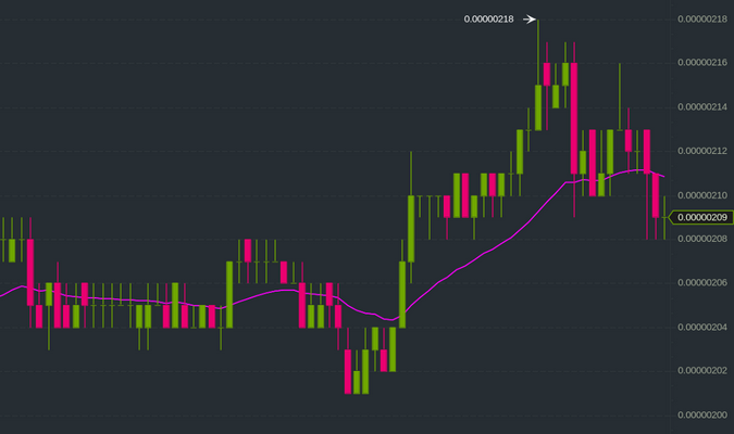
^{TRX/BTC 1-hour candle chart}

The EMA indicator is, in general, a weighted moving average that gives more weight to recent price data. Although a moving average may be a simple indicator, I've had good experiences using it.

The purple line in the chart above shows an EMA-25 indicator (meaning the last 25 values were taken into account).

The bot monitors the pitch between the current EMA-25 value (t0) and the previous EMA-25 value (t-1). If the pitch exceeds a certain value, it signals rising prices, and the bot will place a buy order. If the pitch falls below a certain value, the bot will place a sell order.

The pitch will be the main indicator for making decisions about trading. For this tutorial, it will be called the trade factor.

Toolchain

The following tools are used in this tutorial:

Binance expert trading view (visualizing data has been done by many others, so there's no need to reinvent the wheel by doing it yourself)
Jupyter Notebook for data-science tasks
Pythonic, which is the overall framework
PythonicDaemon as the pure runtime (console- and Linux-only)

Data mining

For a crypto trading bot to make good decisions, it's essential to get open-high-low-close (OHLC) data for your asset in a reliable way. You can use Pythonic's built-in elements and extend them with your own logic.

The general workflow is:

Synchronize with Binance time
Download OHLC data
Load existing OHLC data from the file into memory
Compare both datasets and extend the existing dataset with the newer rows

This workflow may be a bit overkill, but it makes this solution very robust against downtime and disconnections.

To begin, you need the Binance OHLC Query element and a Basic Operation element to execute your own code.

Image by:

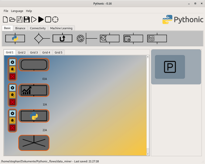
^{Data-mining workflow}

The OHLC query is set up to query the asset pair TRXBTC (Tron/Bitcoin) in one-hour intervals.

Image by:

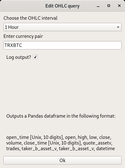
^{Configuring the OHLC query element}

The output of this element is a Pandas DataFrame. You can access the DataFrame with the input variable in the Basic Operation element. Here, the Basic Operation element is set up to use Vim as the default code editor.

Image by:

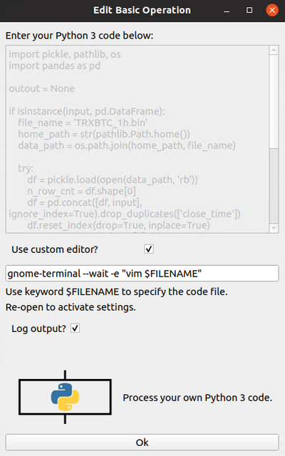
^{Basic Operation element set up to use Vim}

Here is what the code looks like:

import pickle, pathlib, os
import pandas as pd

outout = None

if isinstance(input, pd.DataFrame):
    file_name = 'TRXBTC_1h.bin'
    home_path = str(pathlib.Path.home())
    data_path = os.path.join(home_path, file_name)

    try:
        df = pickle.load(open(data_path, 'rb'))
        n_row_cnt = df.shape[0]
        df = pd.concat([df,input], ignore_index=True).drop_duplicates(['close_time'])
        df.reset_index(drop=True, inplace=True)
        n_new_rows = df.shape[0] - n_row_cnt
        log_txt = '{}: {} new rows written'.format(file_name, n_new_rows)
    except:
        log_txt = 'File error - writing new one: {}'.format(e)
        df = input

    pickle.dump(df, open(data_path, "wb" ))
    output = df

First, check whether the input is the DataFrame type. Then look inside the user's home directory (~/) for a file named TRXBTC_1h.bin. If it is present, then open it, concatenate new rows (the code in the try section), and drop overlapping duplicates. If the file doesn't exist, trigger an exception and execute the code in the except section, creating a new file.

As long as the checkbox log output is enabled, you can follow the logging with the command-line tool tail:

$ tail -f ~/Pythonic_2020/Feb/log_2020_02_19.txt

For development purposes, skip the synchronization with Binance time and regular scheduling for now. This will be implemented below.

Data preparation

The next step is to handle the evaluation logic in a separate grid; therefore, you have to pass over the DataFrame from Grid 1 to the first element of Grid 2 with the help of the Return element.

In Grid 2, extend the DataFrame by a column that contains the EMA values by passing the DataFrame through a Basic Technical Analysis element.

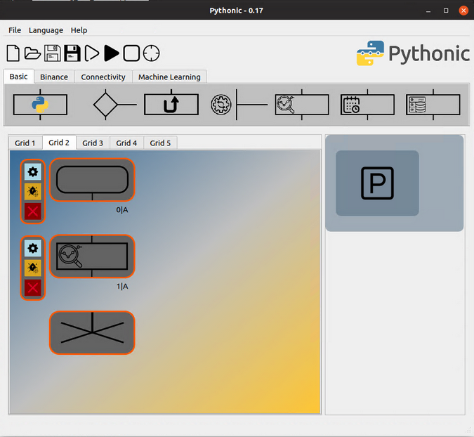
Configure the technical analysis element to calculate the EMAs over a period of 25 values.

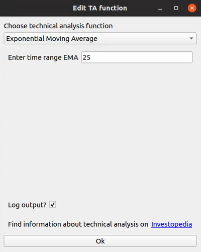
Configuration of the technical analysis element

Image by:

^{Configuring the technical analysis element}

When you run the whole setup and activate the debug output of the Technical Analysis element, you will realize that the values of the EMA-25 column all seem to be the same.

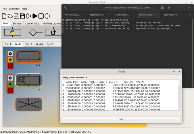
This is because the EMA-25 values in the debug output include just six decimal places, even though the output retains the full precision of an 8-byte float value.

For further processing, add a Basic Operation element:

Image by:

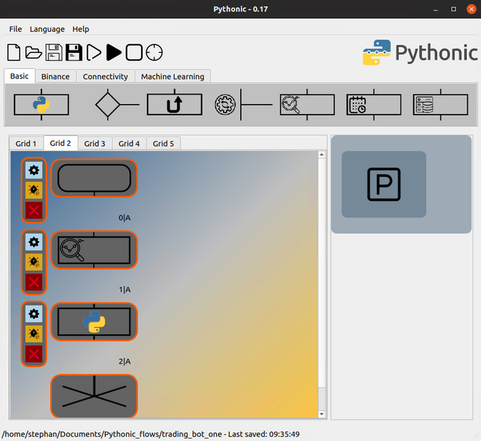
^{Workflow in grid 2}

With the Basic Operation element, dump the DataFrame with the additional EMA-25 column so that it can be loaded into a Jupyter Notebook;

Image by:

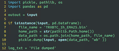
_{Dump extended DataFrame to file}

Evaluation logic

Developing the evaluation logic inside Juypter Notebook enables you to access the code in a more direct way. To load the DataFrame, you need the following lines:

Image by:

^{Representation with all decimal places}

You can access the latest EMA-25 values by using iloc and the column name. This keeps all of the decimal places.

You already know how to get the latest value. The last line of the example above shows only the value. To copy the value to a separate variable, you have to access it with the .at method, as shown below.

You can also directly calculate the trade factor, which you will need in the next step.

Determine the trading factor

As you can see in the code above, I chose 0.009 as the trade factor. But how do I know if 0.009 is a good trading factor for decisions? Actually, this factor is really bad, so instead, you can brute-force the best-performing trade factor.

Assume that you will buy or sell based on the closing price.

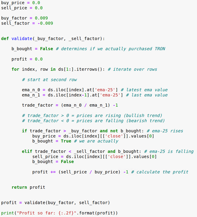
In this example, buy_factor and sell_factor are predefined. So extend the logic to brute-force the best performing values.

Image by:

^{Nested for loops for determining the buy and sell factor}

This has 81 loops to process (9x9), which takes a couple of minutes on my machine (a Core i7 267QM).

Image by:

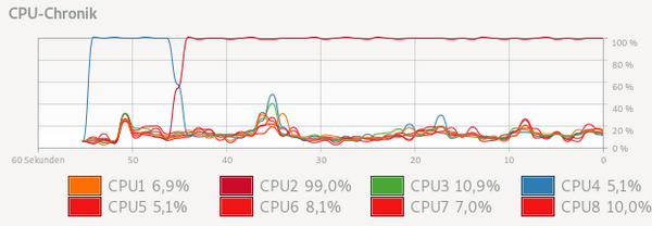
^{System utilization while brute-forcing}

After each loop, it appends a tuple of buy_factor, sell_factor, and the resulting profit to the trading_factors list. Sort the list by profit in descending order.

Image by:

^{Sort profit with related trading factors in descending order}

When you print the list, you can see that 0.002 is the most promising factor.

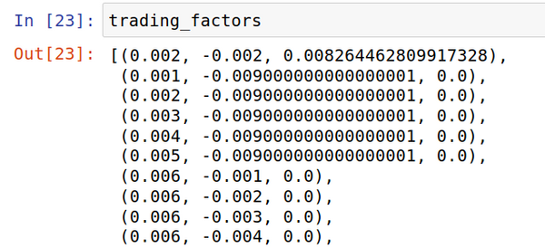
Sorted list of trading factors and profit

When I wrote this in March 2020, the prices were not volatile enough to present more promising results. I got much better results in February, but even then, the best-performing trading factors were also around 0.002.

Split the execution path

Start a new grid now to maintain clarity. Pass the DataFrame with the EMA-25 column from Grid 2 to element 0A of Grid 3 by using a Return element.

In Grid 3, add a Basic Operation element to execute the evaluation logic. Here is the code of that element:

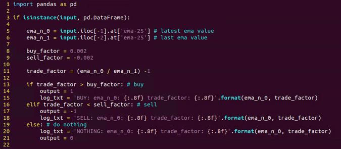
The element outputs a 1 if you should buy or a -1 if you should sell. An output of 0 means there's nothing to do right now. Use a Branch element to control the execution path.

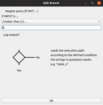
Due to the fact that both 0 and -1 are processed the same way, you need an additional Branch element on the right-most execution path to decide whether or not you should sell.

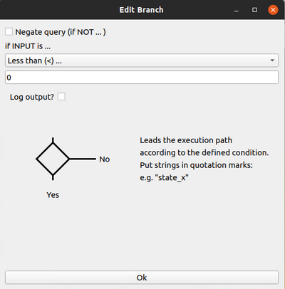
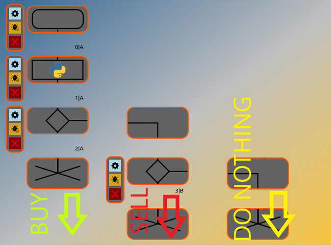
Grid 3 should now look like this:

Execute orders

Since you cannot buy twice, you must keep a persistent variable between the cycles that indicates whether you have already bought.

You can do this with a Stack element. The Stack element is, as the name suggests, a representation of a file-based stack that can be filled with any Python data type.

You need to define that the stack contains only one Boolean element, which determines if you bought (True) or not (False). As a consequence, you have to preset the stack with one False. You can set this up, for example, in Grid 4 by simply passing a False to the stack.

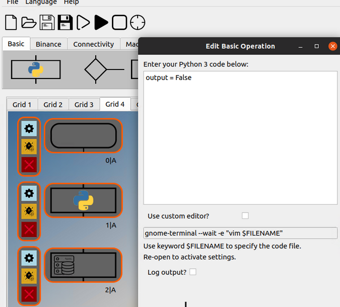
Forward a False-variable to the subsequent Stack element

The Stack instances after the branch tree can be configured as follows:

Image by:

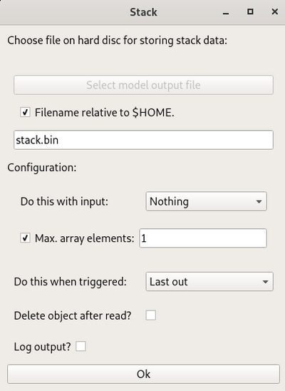
^{Configuring the Stack element}

In the Stack element configuration, set Do this with input to Nothing. Otherwise, the Boolean value will be overwritten by a 1 or 0.

This configuration ensures that only one value is ever saved in the stack (True or False), and only one value can ever be read (for clarity).

Right after the Stack element, you need an additional Branch element to evaluate the stack value before you place the Binance Order elements.

Image by:

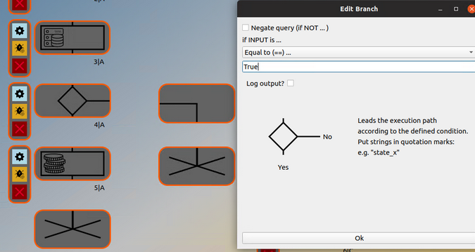
^{Evaluating the variable from the stack}

Append the Binance Order element to the True path of the Branch element. The workflow on Grid 3 should now look like this:

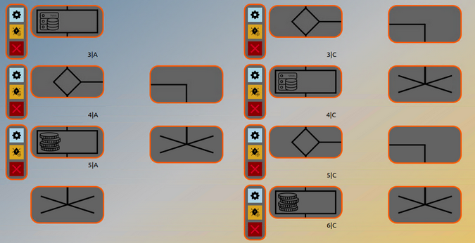
The Binance Order element is configured as follows:

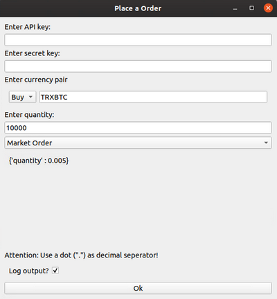
Configuration of the Binance Order element

Image by:

^{Configuring the Binance Order element}

You can generate the API and Secret keys on the Binance website under your account settings.

Image by:

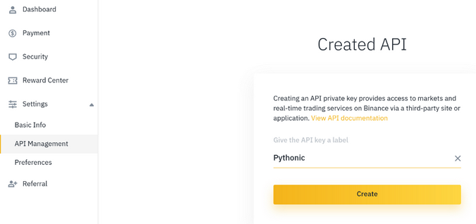
^{Creating an API key in the Binance account settings}

In this tutorial, every trade is executed as a market trade and has a volume of 10,000 TRX (~US$ 150 on March 2020). (For the purposes of this tutorial, I am demonstrating the overall process by using a Market Order. Because of that, I recommend using at least a Limit order.)

The subsequent element is not triggered if the order was not executed properly (e.g., a connection issue, insufficient funds, or incorrect currency pair). Therefore, you can assume that if the subsequent element is triggered, the order was placed.

Here is an example of output from a successful sell order for XMRBTC:

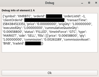
Output of a successfully placed sell order

Image by:

^{Successful sell order}

This behavior makes subsequent steps more comfortable: You can always assume that as long the output is proper, the order was placed. Therefore, you can append a Basic Operation element that simply writes the output to True and writes this value on the stack to indicate whether the order was placed or not.

If something went wrong, you can find the details in the logging message (if logging is enabled).

Image by:

^{Logging output from Binance Order element}

Schedule and sync

For regular scheduling and synchronization, prepend the entire workflow in Grid 1 with the Binance Scheduler element.

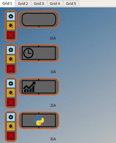
Binance Scheduler at Grid 1, Position 1A

Image by:

^{Binance Scheduler at position 1A, grid 1}

The Binance Scheduler element executes only once, so split the execution path on the end of Grid 1 and force it to re-synchronize itself by passing the output back to the Binance Scheduler element.

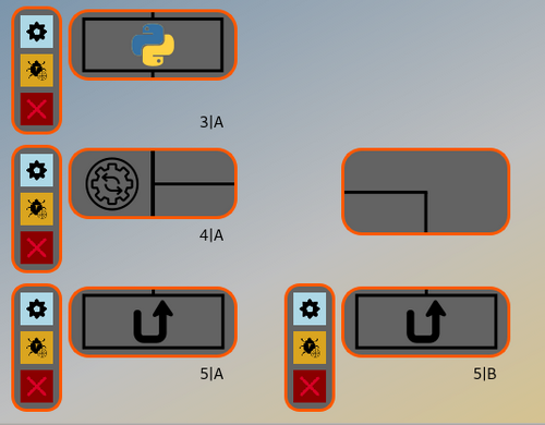
Element 5A points to Element 1A of Grid 2, and Element 5B points to Element 1A of Grid 1 (Binance Scheduler).

Deploy

You can run the whole setup 24/7 on your local machine, or you could host it entirely on an inexpensive cloud system. For example, you can use a Linux/FreeBSD cloud system for about US$5 per month, but they usually don't provide a window system. If you want to take advantage of these low-cost clouds, you can use PythonicDaemon, which runs completely inside the terminal.

Image by:

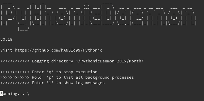
^{PythonicDaemon console}

PythonicDaemon is part of the basic installation. To use it, save your complete workflow, transfer it to the remote running system (e.g., by Secure Copy [SCP]), and start PythonicDaemon with the workflow file as an argument:

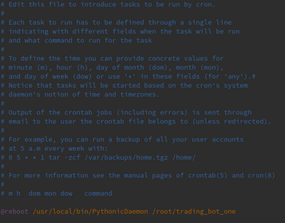
$ PythonicDaemon trading_bot_one

To automatically start PythonicDaemon at system startup, you can add an entry to the crontab:

# crontab -e

Next steps

As I wrote at the beginning, this tutorial is just a starting point into automated trading. Programming trading bots is approximately 10% programming and 90% testing. When it comes to letting your bot trade with your money, you will definitely think thrice about the code you program. So I advise you to keep your code as simple and easy to understand as you can.

If you want to continue developing your trading bot on your own, the next things to set up are: